How COUNTIF function can be used to calculate numbers in Excel
COUNTIF function in Excel is used to count the number of cells in the range in question, the data contained in which meet the criterion passed as the second argument to this function, and returns the corresponding numeric value.
COUNTIFS function can be used to analyze numeric values, text strings, dates, and other types of data. It can be used to determine the number of non-repeating values in a range of cells, as well as the number of cells with data that only partially coincide with the specified criterion. For example, an Excel table contains a column with the full name of customers. To determine the number of namesake customers with the name Jon, you can enter the function =COUNTIF(A1:A300,"*Jon*"). The symbol "*" indicates any number of any characters before and after the substring "Jon".
Examples of using the COUNTIF function in Excel
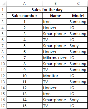
Example 1. The Excel spreadsheet contains data on sales of goods in the hardware store for the day. Determine how much of the Samsung products are sold.
View source data table:
For the calculation we use the formula:
=COUNTIF(C3:C17,"Samsung") / A17
Argument Description:
- C3:C17 is the range of cells containing the names of the companies of the equipment sold;
- "Samsung" - search criteria (exact match);
- A17 is the cell storing the number of the last sale corresponding to the total number of sales.
The result of the calculation:
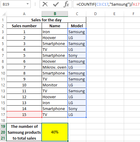
The percentage of Samsung products sold is a percentage of 40%.
Counting the number of a particular cell value in Excel provided
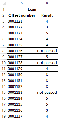
Example 2. According to the results of the exams, it is necessary to create a table containing data on the number of students who passed the subject for 5, 4, 3 points, respectively, as well as those who did not pass the subject.
View source table:
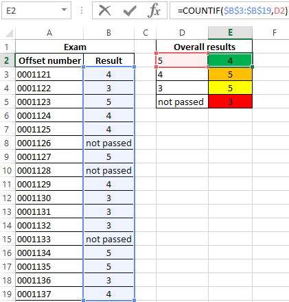
First select the cells E2:E5, enter the formula below:
=COUNTIF(B3:B19,D2:D5)
Argument Description:
- B3:B19 - cell range with exam grades;
- D2:D5 is the range of cells containing the criteria for counting the number of matches.
As a result, we get the table:
Statistical analysis of attendance using the account function in Excel
Example 3. The Excel spreadsheet stores data on page views of the site by the day. Determine the number of users of the site per day, as well as how many times a day users came to the site with default and user_1 logins.
View source table:
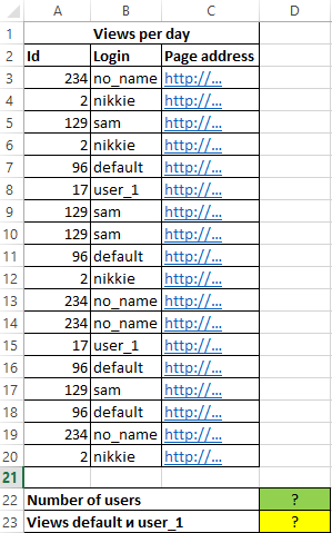
Since each user has his own unique identifier in the database (Id), let's calculate the number of site users per day using the following array formula and to calculate it, press the key combination Ctrl + Shift + Enter:
The expression 1 / COUNTIF(A3:A20,A3:A20) returns an array of fractional numbers 1 / number_notes, for example, for a user with the nickname sam, this value is 0.25 (4 occurrences). The total sum of such values, calculated by the SUM function, corresponds to the number of unique occurrences, that is, the number of users on the site. The resulting value:
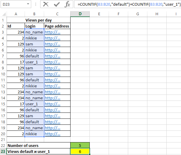
To determine the number of pages viewed by the users default and user_1, we write the formula:
As a result of the calculation we get:
Features of using the COUNTIF function in Excel
The function has the following syntax entry:
=COUNTIF(Range,Criteria)
Argument Description:
- Range - a required argument that accepts a link to one or several cells in which the number of matches with the specified criterion is required to be determined.
- Criteria - the condition according to which the calculation of the number of matches in the considered range is performed. The condition can be a boolean expression, a numeric value, a text string, a Date value, a cell reference.
Notes:
- When counting the number of occurrences in a range in accordance with two different conditions, a range of cells can be considered as a set containing two or more disjoint subsets. For example, in the table "Furniture" you need to find the number of tables and chairs. For calculations, we use the expression =COUNTIF(B3:B200,"*table*")+COUNTIF(B3:B200,"*chair*").
- If a text string is specified as a criterion, it should be noted that the case of characters does not matter. For example, the =COUNTIF(A1:A2,"Joni") function returns the value 2 if the cells "joni" and "Joni" are written in cells A1 and A2, respectively.
- If the criterion is passed as an argument to a reference to an empty cell or an empty string "", the result of the calculation for any range of cells will be the numeric value 0 (zero).
- The function can be used as an array formula if you need to calculate the number of cells with data that satisfies several criteria at once. This feature will be considered in one of the examples.
- The function in question can be used to determine the number of matches, either one at a time or according to several search criteria at once. In the latter case, two or more COUNTIF functions are used, the returned results of which are added or subtracted. For example, cells A1:A10 store a sequence of values from 1 to 10. To counting cells with numbers greater than 3 and less than 8, you must perform the following steps:
Download examples COUNTIF function for counting of cell in Excel
- write down the first function of COUNTIF with criterion ">3";
- write the second function with the criterion ">=8";
- to determine the difference between the returned values =COUNTIF(A1:10,">3")-COUNTIF(A1:A10,">= 8"). That is, subtract from the set (3,+∞) the subset [8,+∞).
