COUNTIFS function calculates count of cells by condition in Excel
The COUNTIFS function is designed to count the number of cells from a range that satisfy one or more criteria, and returns the corresponding numeric value. Unlike the COUNTIF function, which takes only one argument with a data selection criterion, the function in question allows you to specify up to 127 criteria.
Examples of using the COUNTIFS function in Excel
With the COUNTIFS function, you can calculate the number of cells that meet the criteria applicable to a column with numeric values. For example, cells A1:A9 contain a number series from 1 to 9. Function = COUNTIFS(A1:A9,">2"A1:A9,"<6") returns 3 because there are 3 numbers between numbers 2 and 6 ( 3, 4 and 5). Also, data selection criteria can be applied to other columns of the table.
How to calculate the number of positions in the price list by the condition?
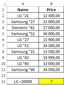
Example 1. Determine the number of LG-made TVs in the data table, the value of which does not exceed 20,000.
View source table:
To calculate the number of LG TVs, the cost of which does not exceed 20,000, we use the following formula:
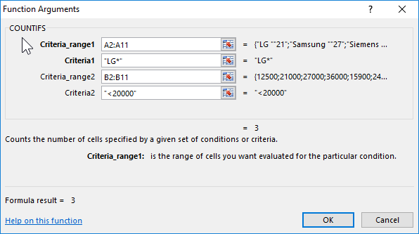
Argument Description:
- A2:A11 - the range of the first condition, the cells of which store text data with the company name and the diagonal value;
- "LG *" - search condition with the wildcard "*" (any number of characters after "LG";
- B2:B11 - the range of the second condition, containing the value of the goods;
- "<20000" is the second search term (price is less than 20,000).
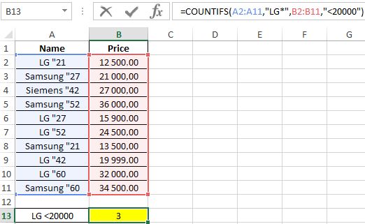
Result of calculations:
How to calculate the share of a group of products in the price list?
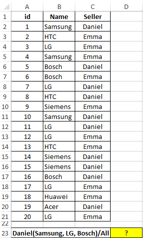
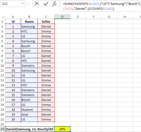
Example 2. The table contains data on purchases in the online home appliances store for a certain period of time. Determine the ratio of LG, Samsung and Bosch products sold by the seller with the last name Ivanov to the total quantity of goods sold by all sellers.
View source table:
To obtain the desired value, we use the formula:
To search for several values at once in the data vector (column B: B), the argument of condition1 was the array constant {"LG","Samsung","Bosch"} therefore, the formula must be executed as an array formula. The SUM function counts the number of elements contained in the array of values returned by the COUNTIFS function. The COUNT function returns the number of non-empty cells in the A2: A21 range, that is, the number of rows in the table. The ratio of the obtained values is the desired value.
As a result of the calculations we get:
How to count the number of cells for several conditions in Excel?
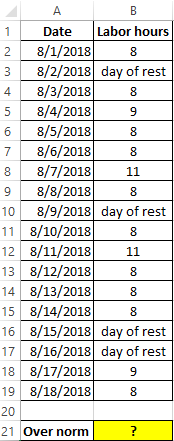
Example 3. The table shows data on the number of hours worked by an employee over a period of time. Determine how many times an employee has worked in excess of the norm (more than 8 hours) in the period from 08/03/2018 through 08/14/2018.View of data table:
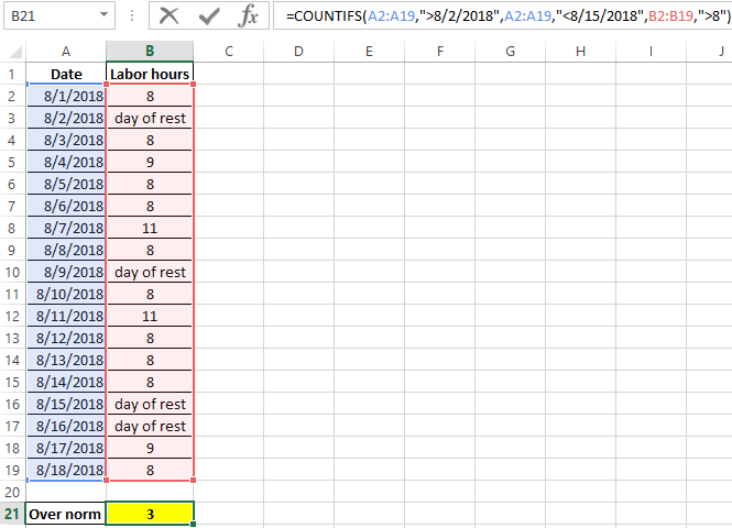
For calculations, use the following formula:
The first two verification conditions are dates that are automatically converted to an Excel time code (numeric value), and then the verification operation is performed. The last (third) criterion - the number of working hours is more than 8.
As a result of calculations, we obtain the following value:
Features of using the COUNTIFS function in Excel
The function has the following syntax entry:
=COUNTIFS(Criteria_range1,Criteria1,[condition_ range2,condition2],...)
Argument Description:
- Criteria_range1 is a required argument that accepts a reference to a range of cells for which the criterion specified in the second argument will be applied to the data contained;
- Criteria1 is a required argument that accepts a condition for selecting data from a range of cells specified as a range_condition1. This argument takes numbers, data of a reference type, text strings containing logical expressions. For example, from the table containing the fields “Name”, “Cost”, “Screen diagonal” you need to select devices whose price does not exceed $ 1,000, the manufacturer is Samsung, and the diagonal is 5 inches. As conditions, you can specify “Samsung *” (the wildcard “*” replaces any number of characters), “> 1000” (price over 1000, the expression must be specified in quotes), 5 (exact numerical value, quotes are optional);
- [range_condition2; condition2]; ... - a pair of subsequent arguments of the function in question, the meaning of which corresponds to the arguments range_condition1 and condition1, respectively. Up to 127 ranges and conditions for selecting values can be specified.
Download examples COUNTIFS function calculates in Excel
Notes:
- In the second and subsequent condition ranges ([condition_range2], [condition_range3], etc.), the number of cells must correspond to their number in the range specified by the condition_range1 argument. Otherwise, the COUNTIFS function will return the error code #VALUE !.
- The function in question checks all the conditions listed as condition1, [condition2], and so on, for each row. If all conditions are met, the total amount returned by COUNTIFS is increased by one.
- If the condition N argument was passed to a reference to an empty cell, the conversion of the empty value to a numeric 0 (zero) is performed.
- When using textual conditions, you can set inaccurate filters with the wildcard characters "*" and "?".
