Download examples of using the FIND function in Excel
The FIND function looks for the value in a sentence or phrase with a phrase and returns the result - a serial number. The item of the value from which the search for the specified character in the found string begins is an optional argument.
Practical work of the FIND function in Excel
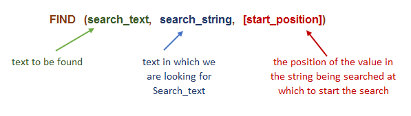
About the FIND function. Schematically, its syntax can be illustrated in the following way:
The third argument is used depending on the task. When a function has only two arguments, the third one defaults to one. If the search_text is not found, the #VALUE! (error) is returned. When there is no match for the search element, the result is an error. This one works exactly like SEARCH, they have the same syntax. Despite this, they have some differences in their work, for example, FIND works correctly if you specify the same register of the desired value and the value being viewed. In the picture we see text where one word is used in different registers. In the first situation, we need to find the word in lower case, and in the second case, in upper case:
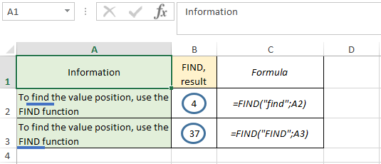
We have different result – its «4» for the first example and «37» for the second one. Now let's see how SEARCH works with the same arguments:
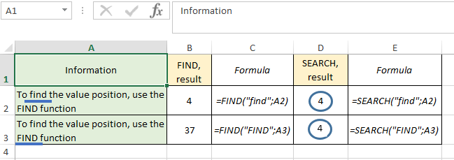
Now we observe the main difference in the performance of the task of the two compared functions - both for the first and for the second situation, the result is "4", since SEARCH does not respond to different registers. Also, this The function does not work correctly with wildcards such as "*", "?", "~":
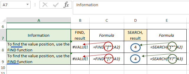
However, this doesn’t apply to SEARCH, which returns us the correct result.
Practical examples of how formulas work to FIND a value
How to use FIND formulas with other IFERROR, REPLACE, LEFT, RIGHT, MID, LONG, SUM, NUMBER functions in Excel? Consider an example in which we will combine FIND and REPLACE. Below we will try to replace the word "song" with "poem":
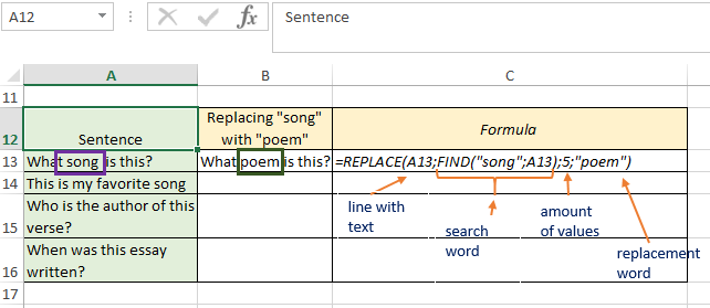
Cell A8 is the cell that contains the phrase and word to be replaced. In place of the second argument, put FIND to find out where the word is placed. We needed this, since the exact location of the “song” is unknown (with what item the word begins). The number 5 indicates the number of characters that we will replace (the number of letters in the word "song"). In this example, we have the same number of characters of the search and replacement text, but this is not a prerequisite, the difference can be any.
Copy the formula to the end of the column:
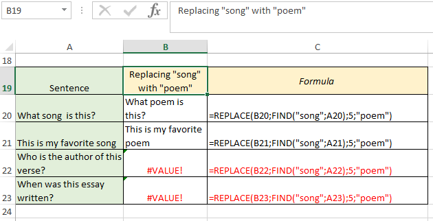
In cell B21, we also replaced the value, and below we returned errors, since the word specified by the condition was not found in the search texts. For the correct display of the result, we indicate that in case of an error, let the same sentence from column A be displayed (without changes). For this we use IFERROR. Its first argument will be the entire previous formula, and the second - a cell from column A:
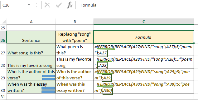
In column B, at the place of error, identical sentences from column A are received.
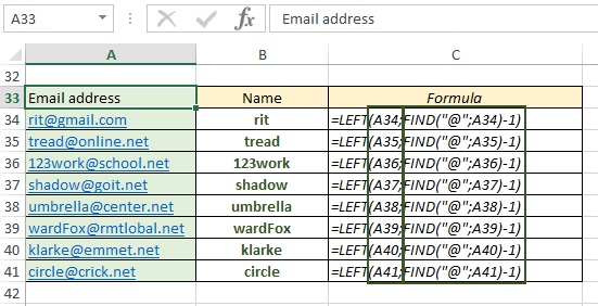
The FIND function is also often used alongside the LEFT, RIGHT, and MID functions to extract part of a phrase. For example, we have a list of email addresses. We need to extract the username (the part before the @ symbol). To complete the task, use the LEFT. As the first argument, we will have a cell with contents, and the second is the FIND function with the prefix "-1", which returns the position of the @ sign and takes a step back (we need this so that the result does not extract the character itself):
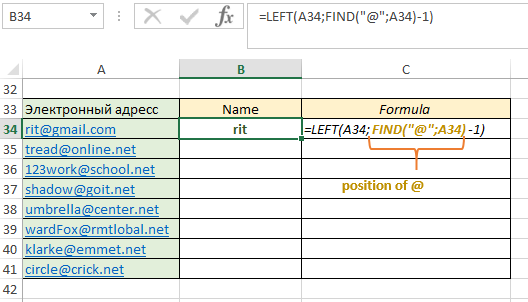
First, the FIND formula returned us the value "4" - this is the position of the desired character. FIND - 1 = 3. Then LEFT extracted three characters to the left side - rit. Copy the formula to the end of the column:
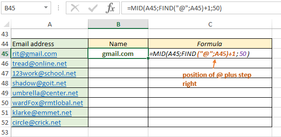
Now let's define the following task: we need to extract the domain name. To implement it, we additionally use the MID function. MID will allow you to consider a substring from any place to the end. The +1 prefix will indicate that the extraction occurs from the next character from @. In this case, we need to specify a number in place of the third argument, which, as we are sure, will be exactly greater than the length of the text string. In this example, we use 50 (it is unlikely that there is an e-mail whose name contains more than 50 characters):
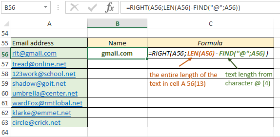
There is another way to solve this problem. This time we use LEN and RIGHT. The basis will be RIGHT. The first argument to RIGHT will be the cell with the search text, and the second argument will be the difference between LEN and FIND. LEN returns the number of characters in a text string:
Copy the formula to the end of the column and get the result:
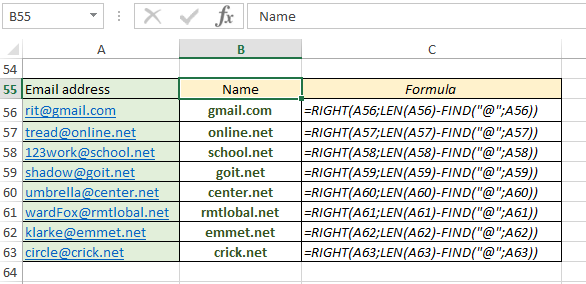
We have completed the task, but the first method is much easier, shorter and clearer. However, the second method is useful in order to better understand the possibilities of combining functions, how they work together and how they can be used for different tasks.
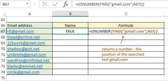
In order to determine the presence of a substring, you can additionally use the ISNUMBER function. The principle of operation is as follows: if FIND returns the position number of the character, then ISNUMBER indicates the value "TRUE", and if it returns an error, indicates "FALSE". For example, let's take a list with email and check if gmail.com is among them:
Copy the formula to the end of the column and check the result:
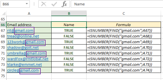
As you can see, in front of the text where the desired value was "gmail.com", we got the result TRUE. The formula above evaluates the contents of a cell. Some users may have thought to use the boolean IF, but it looks for an identical match of the given search text, "gmail.com" equals "gmail.com", and we need "gmail.com equals "position number". Then ISNUMBER will determine the presence or absence of a number, and return the result.
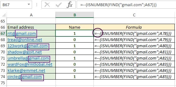
You can transform the function above by adding two dashes in front of the ISNUMBER. Thus, it will count the number of results: for TRUE it will return one, and for FALSE it will return zero:
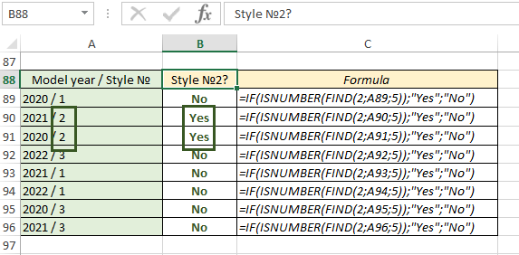
You can make the formula even more complex by using an additional IF and customizing the answers you want. In the example, the table provides the model year and style number. IF evaluates a logical operator and returns "Yes" if TRUE and "No" if FALSE:
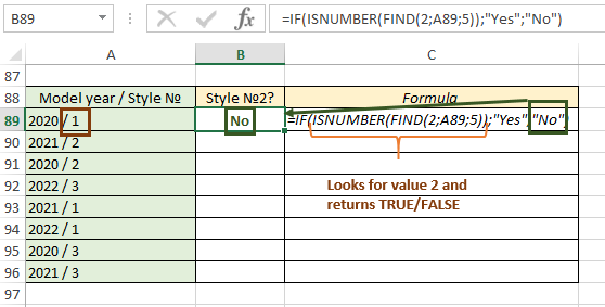
This time we've added a third argument, the number 5, which indicates where the search starts. Since the model year also contains the lookup value "2", we specified that the lookup must occur exactly from the style number. Copy the formula to the end of the column and check how the formula worked. The phrase "Yes" appeared in front of those cells whose style number is 2:
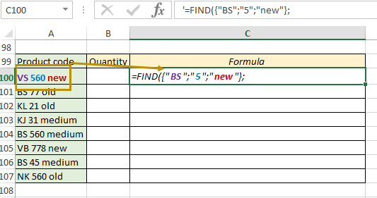
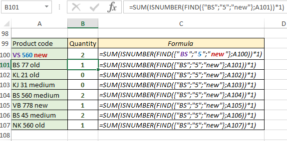
Now consider an example where we need to calculate the sum of the found values at the same time. To do this, you need to add SUM. In cell A100 we have three elements - an alphabetic code, a numeric code, a word. We need to find out if the first element is BS, the second is the number 5, and the third is the word “new”. Since the search text now contains three values instead of just one, it is an array that we need to put in brackets {}:
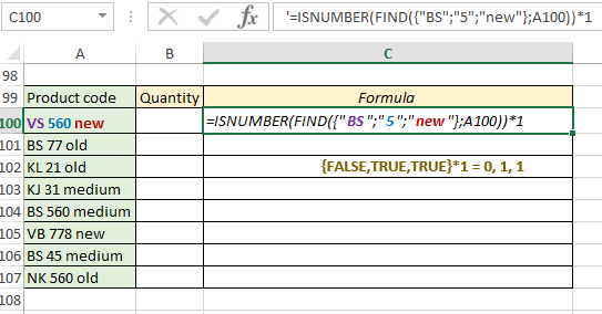
Right now, a content in parentheses its an array of three elements. That means, we need to find these items in A100. Our function three times will looks for elements like a circle for every of them. Then we add an A100 to start the search. We place the built formula in ISNUMBER. At this point, the get the next result: the first one is FALSE, the second one is TRUE and the third one is TRUE. And we need to convert them to numbers. To do this, add the prefix "*1" to the ISNUMBER. TRUE * 1 is equal to 1, FALSE * 1 is equal to 0:
Now we just need to calculate the data. To do this, we put what we got in the SUM, press Enter:
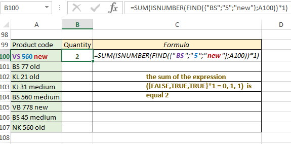
We apply the constructed formula throughout the list:
 Download examples of using the FIND function in Excel
In cell A101, only one BS element matches, the sum of the elements is 1.
