Download example SUMIFS with dates many conditions in Excel

SUMIFS is a mathematical formula. It sums up the cells that match the given conditions. It works the same way as the SUMIFS function, the difference is that SUMIFS can use many conditions to work with any values: dates, number or text.



How the SUMMESLIMN function works in Excel

Its syntax looks like this:

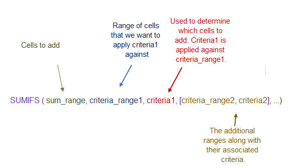
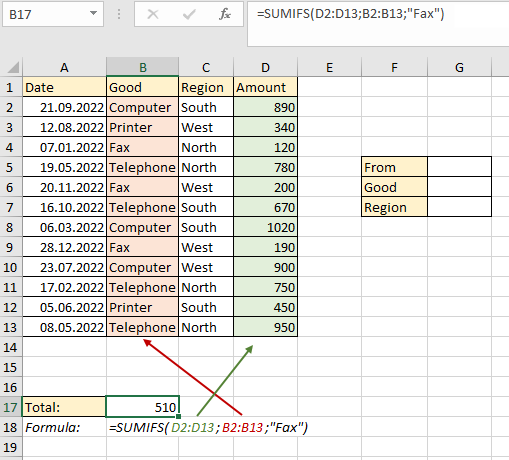
There is also another difference between similar functions. In the picture, we can see that the "Conditions" argument takes the 3rd place, and for SUMMIF it is the first argument. Let's move on to practical examples. We have a table with data that contains information about the sale of goods in certain regions, there is also a date of sale and an amount. Let's take a look at the arguments first. To do this, let our first task be to calculate the amount of fax sales. In cell B17, we start writing the formula. Select the cells D2:D13 - the summation operation will be carried out on it. Then select the data set of criteria B2:B13 - it will match the condition. After that, in quotation marks, we indicate the product "Fax" - this is our condition:

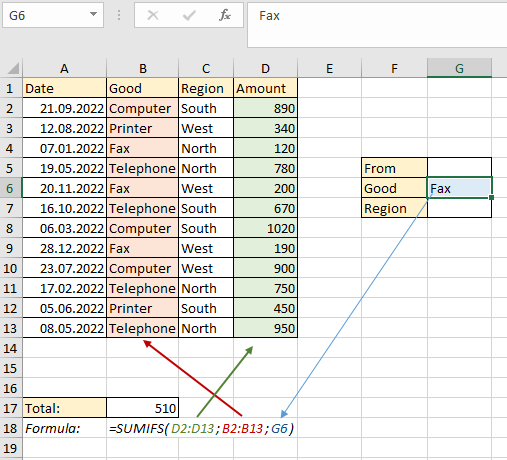
In order not to use text in the formula, but to use a cell reference, we will enter the data we need in the table on the right. Enter the text "Fax" in cell G6 and use the reference to it in the SUMIFS formula:

But this simple task can also be implemented with the help of SUMMESLI, only the order of the arguments will change. Now let's make changes to the initial conditions of the problem. Now we need to find the amount of fax sales in the north. We enter the data in the table on the right and build our formula, referring to the cells:

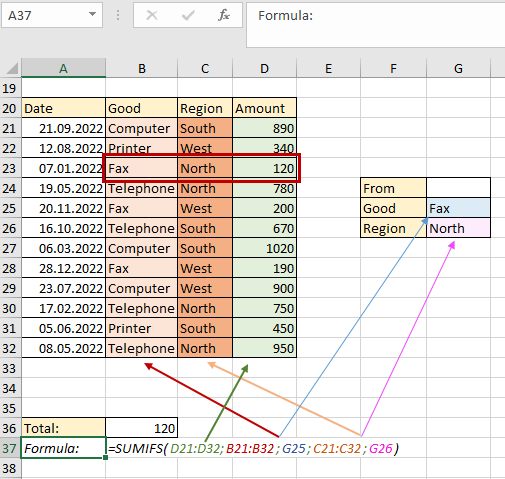
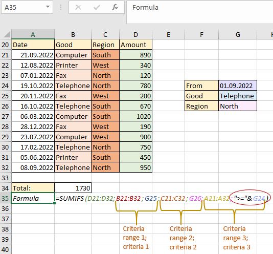
The first argument is a column with the sum, the second is the range in which matches are searched for condition No. 1, the third is condition No. 1, the fourth is the data in which matches are searched for condition No. 2, the fifth is condition No. 2. That is, first we select the data set of the final summation, and then as many conditions and ranges as we want that contain these conditions. Now let's add a final condition so that the formula selects the sum of phone sales in the north since September. There is a feature here: for the last argument. In cell G24, we indicate the date 09/01/2022, and in the formula we indicate that we need to look for the amount after (greater than, “>=”) the specified date. In order for the formula to work correctly, you need to connect the operator and the cell through an ampersand (&):

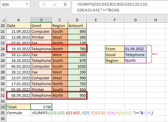
Now SUMIFS accepts three conditions and will calculate the amount that will match all three criteria from the table on the right. Under these conditions, the amount from series No. 24 and No. 32 is suitable:

The previous examples of tasks worked according to the principle “and criterion 1, and criterion 2, and criterion 3”, that is, they found a common element that would meet all three given conditions at the same time. That is, we can say that the syntax of the formula itself implies the use of the AND operator. Now let's look at an example where we will implement a scenario in which the formula will count those elements that match several criteria in one column of the criterion data.



Example of an SUMIFS with many conditions in one Excel column

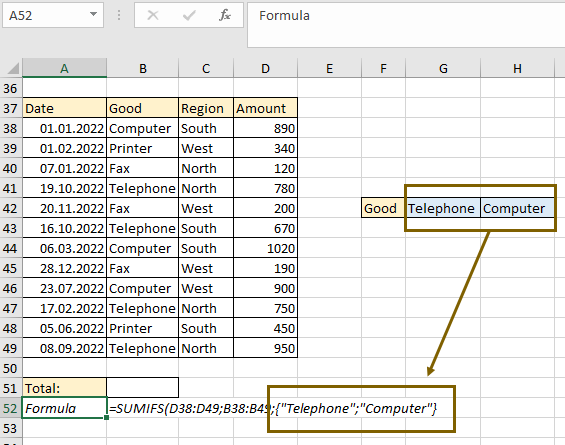
We need to calculate the total amount of sales of phones and computers. To do this, we first construct the SUMIFS formula. The first argument is, as usual, the summation range, the second is the data set of criteria. For the third argument, we will specify two criteria in text form in curly brackets - "phone", "computer":

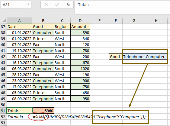
But since it's an array now, we need to add a SUM formula to make it count the values from the array. We get the desired result:

Thus, you can add as many criteria as you need. Such a formula works according to the logic of using the "OR" operator. You can also add another range of criteria and a condition for it. For example, for the "Region" range, add the value "South". That is, we need to find the sum of sales of phones or computers in the south:

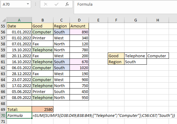
It is important not to get confused in the order of the arguments. First, as always, we specify the summation range, then the first range of criteria, then the array of criteria. After that, if there are additional conditions, we specify the second range of criteria and the second single argument or array of arguments. As a result, we returned the value of the sum of sales of phones or computers in the south - 2580. Now let's add one more condition to the second condition to get an array of criteria not only in the first part of the formula, but also in the second. In addition to the south, we will also search in the west:

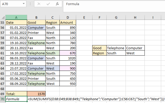
Now, as a result, we have returned the amount of 1570. How did the formula work? First, the function selected values by phones and computers. Then, for the phone, she selected the amount for the "South" region, and for the computer - for the "West" region. Between the two arrays of conditions, the function drew parallels in the order in which they are. If we were to swap the words "South" and "West", then we would get the following meaning:

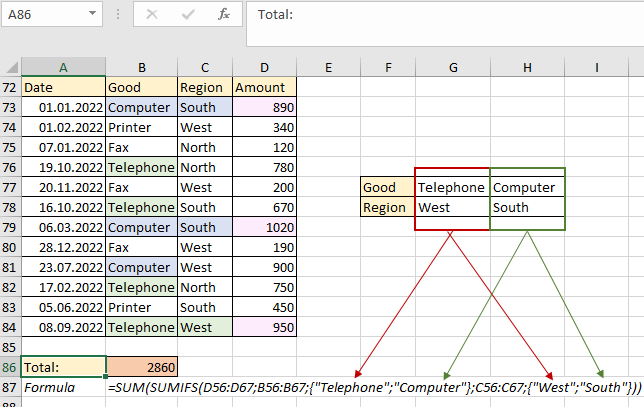
That is, the formula works on pairs of criteria from the first and second arrays. A very handy feature if you need to select products that match several characteristics at the same time.

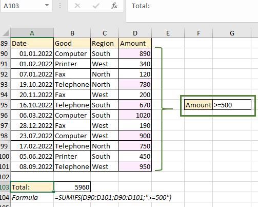
In the following example, we need to sum those values whose sum is greater than or equal to 500. In this case, the first and second arguments will be identical, since it contains both the condition and the summed values. Then we add the third argument. Since the ">=500" argument is text, we need to use quotes:

But since SUMIFS allows us to use multiple conditions, let's create a table with conditions so that we can refer to cells and make our formula dynamic, and add the following condition: "Items sold after September 1, 2022":

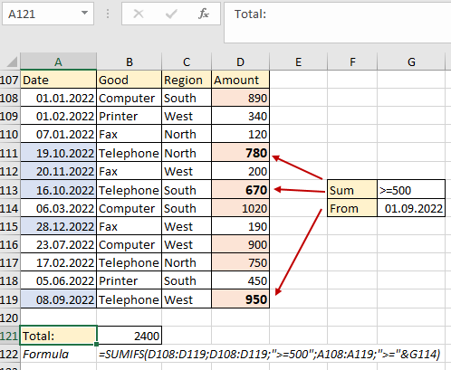
The formula first found those numbers that are greater than 500, then selected those that met the second criterion - greater than or equal to the specified date. Thus, SUMIFS selected three suitable values, summed them up, and returned the result 2400. Also in this example, an ampersand was used, which is necessary to connect the text value "greater than equals" and the cell reference. In the following example, we will use two tables and see how convenient it is to work with them using the SUMIFS function in two ways.

Using SUMIFS with dates in Excel

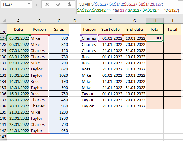
In the second table, we have the criteria specified correctly, so you can immediately refer to the cells. In cell H126, we begin to build a formula: the first criterion is a range with sales, the second is a range with names from the first table, and the third is the name "Charles" from the second table. Then we add another range of conditions - the date column from the first table. Also, now we need to add another set of conditions and ranges - after the start date and before the end date. Be sure to use absolute references for ranges, because we will copy the formula. It will look like this:

We copy the formula to the end of the column and get the results for sales for three periods by name:

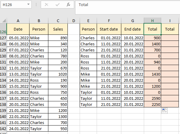
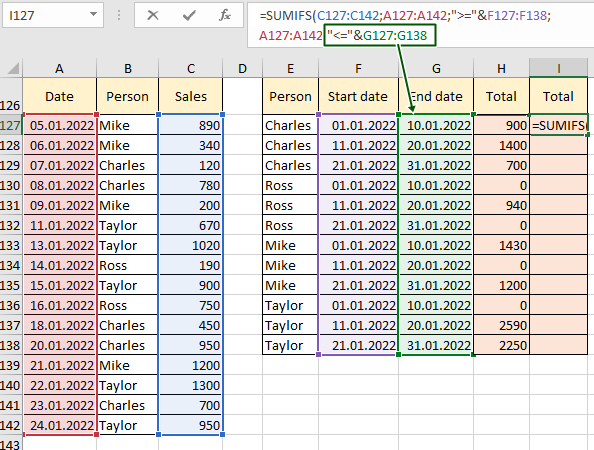
Now we have specific information that displays real data. For example, we see that some employees did not make sales in certain periods - their result is zero. But there is another way we can change our formula. This time we use the condition not unique, but range. We begin to build the formula step by step. As before, the first argument is the "Sales" range. After that, select the "Date" range. Now we need to specify the boundaries of the period again through the operators "greater than", "less than", "equal to". We print ">="& and now we need to select not a cell with a condition, but a range of conditions F127:F138:

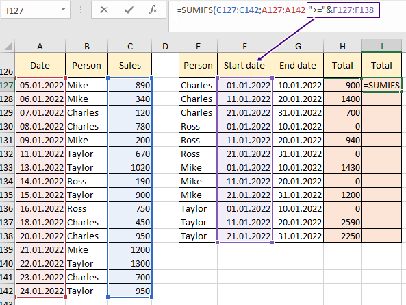
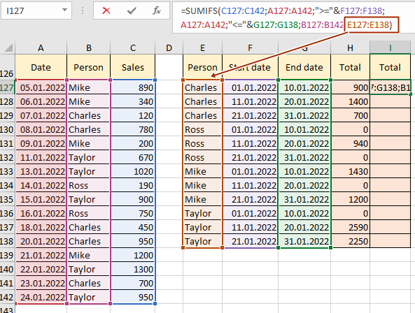
Now we do the same for one more condition. Add the "Date" criteria range, add the text value "<=" and add the end date range G127:G138 through the ampersand:

Now it remains to add the last range of person conditions from the second table and the range of conditions for searching for persons from the first table:

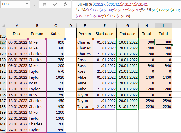
Press Enter, where necessary, specify absolute links so that the cells do not slide down and get the result for all names:

Download all the examples of AMMESLIMN with dates if there are many conditions in Excel

The order of ranges with conditions can change. The main rule is that the summation range should be argument No. 1, so the name and boundaries of the periods can be specified in any order, but must be paired with the search range of the corresponding criterion.