Examples of the ADDRESS function for getting the cell address of an Excel sheet
ADDRESS function returns the address of a specific cell (text value) pointed to by the column and row numbers. For example, as a result of the function =ADDRESS(5;7), the value of $G$5 will be displayed.
Note: the presence of "$" characters in the $G$5 address indicates that the reference to this cell is absolute, that is, it does not change when copying data.
ADDRESS function in Excel: syntax features description
ADDRESS function has the following syntax entry:
=ADDRESS(Row_num, Column_num, [Abs_num], [A1], [Sheet_text])
The first two arguments of this function are required.
Argument Description:
- Row Number is a numeric value corresponding to the line number in which the required cell is located;
- Column number is a numeric value that corresponds to the column number in which the desired cell is located;
- [Abs_num] is a number from the range from 1 to 4, corresponding to one of the types of the returned cell reference:
- Absolute on all cell, for example - $A$4.
- Absolute only per line, for example - A$4.
- Absolute only per column, for example - $A4.
- Relative to the whole cell, for example A4.
- [A1] is a logical value that defines one of two types of links: A1 or R1C1;
- [Sheet_text] is a text value that defines the name of a sheet in an Excel document. Used to create external links.
Notes:
- References of type R1C1 are used to number columns and rows. To return links of this type, the logical value FALSE or the corresponding numeric value 0 must be explicitly specified as the a1 parameter.
- The link style in Excel can be changed by checking / unchecking the checkbox of the menu item “Link style R1C1”, which is located in “File - Options - Formulas - Working with Formulas”.
- If you need a reference to a cell that is located in another sheet of this Excel document, it is useful to use the [sheet_name] parameter, which takes a text value that corresponds to the name of the desired sheet, for example, "Sheet7".
Examples of using ADDRESS function in Excel
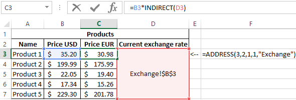
Example 1. The Excel spreadsheet contains a cell that displays dynamically changing data depending on certain conditions. To work with the actual data in the table, which is located on another sheet of the document, you need to get a link.
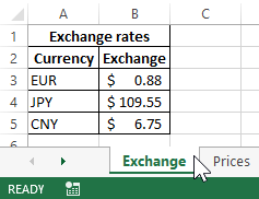
On the sheet "Exchange" created a table with the current exchange rates:
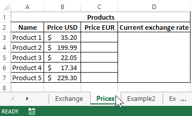
On a separate sheet “Prices”, a table with goods was created, displaying the value in US dollars (USD):
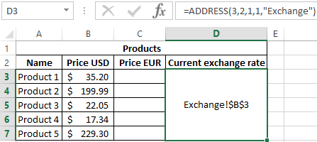
In D3 we place a link to a cell in the table located on the sheet “Exchange”, which contains information about the USD exchange rate. To do this, we introduce the following formula: =ADDRESS(3;2;1;1;"Exchange").
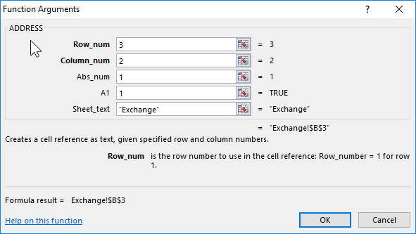
Parameter value:
- 3 - the number of the line containing the required cell;
- 2 - the column number with the desired cell;
- 1 - reference type is absolute;
- 1 - select the style of links with alphanumeric entry;
- “Exchange” is the name of the sheet on which the table with the desired cell is located.
To calculate the cost in Euro, we use the formula: =B3*INDIRECT(D3).
INDIRECT function is required to obtain a numeric value stored in the cell referenced. As a result of calculations for other products, we obtain the following table:
How to get the ADDRESS of the cell reference Excel?
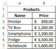
Example 2. The table contains data on the price of goods, sorted in ascending order of value. It is necessary to get links to cells with the minimum and maximum cost of goods, respectively.
The source table is as follows:
To get the reference to the cell with the minimum cost of the goods use the formula:
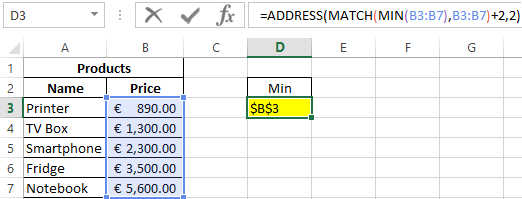
ADDRESS function accepts the following parameters:
- The number corresponding to the line number with the minimum price value (the MIN function searches for the minimum value and returns it; the MATCH function finds the position of the cell containing the minimum price value. Added 2 to the resulting value, because the MATCH searches for the range of selected cells.
- 2 - the number of the column in which the desired cell is located.
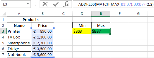
In a similar way we get a link to the cell with the maximum price of the goods. As a result, we get:
ADDRESS by row and column numbers of an Excel sheet in the style of R1C1
Example 3. The table contains a cell, the data from which is used in another software product. To ensure compatibility, you must provide a link to it in the form of R1C1.
The source table is as follows:
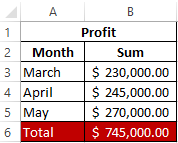
To get a reference to B6, we use the following formula: =ADDRESS(6;2;1;0).
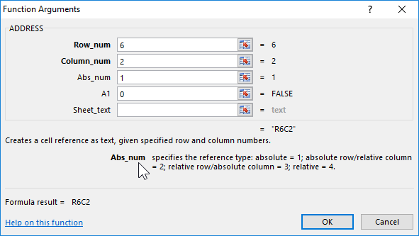
Function Arguments:
- 6 - line number of the desired cell;
- 2 - the number of the column containing;
- 1 - type of reference (absolute);
- 0 - an indication of the style R1C1.
As a result, we get the link:
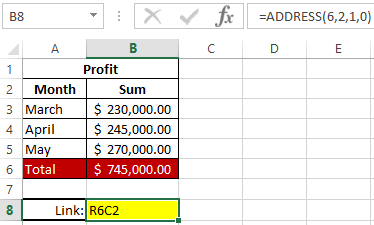
Practical application of the ADDRESS function: Searching of the value in a range Excel table in columns and rows.
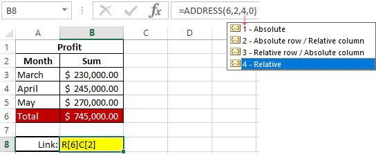
Note: when using the R1C1 style, the absolute reference record does not contain the "$" sign. To distinguish between absolute and relative references, square brackets "[]" are used. For example, if in this example, as the type of link parameter, specify the number 4, the cell reference will look like this:
Download examples ADDRESS function for getting link to cell in Excel
This is the absolute type of links in rows and columns when using the R1C1 style.
