How to use the SUM formula in Excel with examples
The SUM function concern into the category «Mathematical». Press the combination of hot keys SHIFT + F3 to call of the function wizard, and you will quickly search out it there.
The using of this function significantly expands to the possibilities of the process of summing the values of the cells in Excel. We look at the possibilities and settings for the summing several ranges practically.
How in the Excel table to calculate the amount of the column?
Sum up the value of the cells A1, A2 and A3 using the summation function and at the same time we will learn what the sum function is used for.
- After entering the numbers, go to the cell A4. On the «Home» tab, select the «Sum» tool in the «Edit» section (or press the ALT + = hot keys combination).
- The range of the cells is recognized automatically. The reference addresses are already entered in the parameters (A1:A3). The user only remains to press Enter.
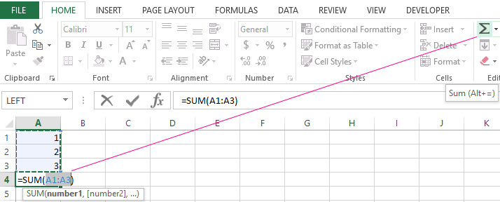
Consequently, the calculation result is displayed in the cell A4. The function itself and its parameters can be seen in the formula bar.
The notation. Instead of using the «Sum» tool on the main panel, you can directly enter the function with parameters manually in the cell A4. The result will be the same.
The Automatic Range Recognition Correction
When you enter of the function using the button on the toolbar or using the function wizard (SHIFT + F3), the SUM () function refers to the group of formulas «Mathematical». Automatically recognized ranges are not always suitable for the user: its can be quickly and easily repaired if necessary.
Suppose we need to sum several ranges of cells, as shown in the picture:
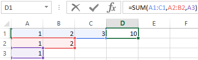
- Go to the cell D1 and select the «Sum» tool.
- While holding the CTRL key, select the range A2:B2 and the cell A3.
- After selecting of the ranges, press Enter and in the cell D4 immediately displays the result of summing the values of cells in all ranges.
Pay attention to the syntax in the function parameters when selecting multiple ranges, that are divided among themselves (;).
In the SUM formula parameters may contain:
- the links to individual cells;
- the references to ranges of the cells both contiguous and non-adjacent;
- the integer and fractional numbers.
In the function parameters, all arguments must be separated by a semicolon.
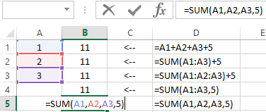
For the illustrative example, let's consider different variants of summation of values of cells, that give the same result. To do this, fill the cells A1, A2 and A3 with numbers 1, 2 and 3 respectively. And fill the range of the cells B1:B5 with the following formulas and functions:
For any variant, we get the same result of calculation - the number 11. Continue successively with the cursor from B1 and to B5. In each cell, press F2 to see the color highlighting of the links for a more intuitive analysis of the syntax for writing parameters.
The contemporaneous summation of the columns
In Excel, you can simultaneously sum several adjacent and non-adjacent columns.
Fill in the columns, as shown in the picture:
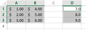
- Select the range A1:B3 and holding down the CTRL key also select the column D1:D3.
- On the «HOME» panel, click the «Sum» tool (or press ALT + =).
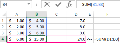
Under each column, the SUM () was automatically added. Now in the cells A4;B4 and D4 the result of the summation of each column is displayed. This is the fastest and most convenient method.
The notation. This function automatically substitutes the format of the cells it sums.
