Examples of INDEX functions step-by-step download in Excel

The INDEX function helps you retrieve a value from an array of data. An array can differ in its structure, the number of columns and rows, and even the number of arrays themselves can be more than one.

An example of the INDEX function in Excel from simple to complex

Let's look at the simplest application example first. We have several cities. Let our first task be to extract the fifth city from our one-dimensional database. The syntax of our formula will be the following: INDEX(array; row_number). We start writing the formula (cell B9). The first argument is all cities B3:C7, and the second is the number of the row we need, which stores the information we want to receive - the fifth city:

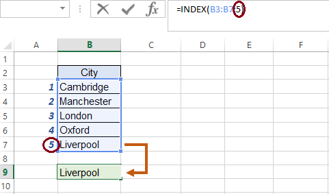
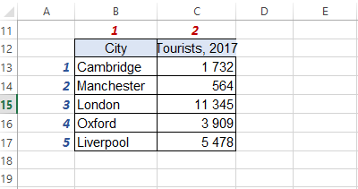
The function returned the value from the second row of our table. Now let's supplement our table with information about tourists who visited the city in 2017:

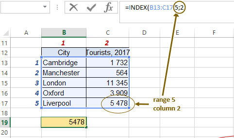
Now our array is two-dimensional. Let the current task be to find out how many tourists visited Liverpool. In cell B19 we write the formula.

INDEX function two-dimensional and multidimensional array

The syntax will also change: INDEX(array; row_number; column_number), we will add a third argument - the number of the column in which the data we need is stored:

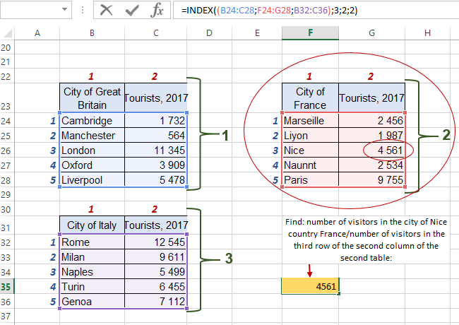
Similarly, the function works with three-dimensional arrays, four-dimensional, and so on. Now let's look at how to solve problems when there are many tables. Let us have cities of three countries with the amount of visitors:

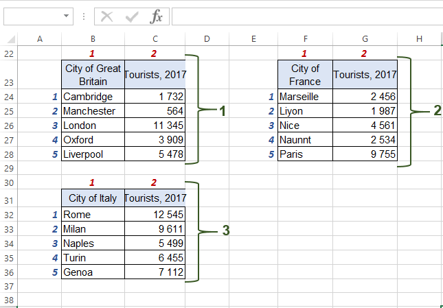
This time we have three two-dimensional tables - three countries with different cities and their visitors. We need to find the number of tourists in the city of Nice in the country of France OR, to paraphrase our syntax, the number of visitors in the third row of the second column of the second table. First of all, as before, we need to select a range. BUT now we have three of them, which means that we choose all three, having previously taken this part of the syntax into brackets. Then we add the coordinates of the information we are looking for already familiar to us - the row and column and the number of the table that contains the range we are looking for:

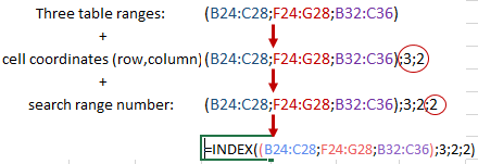
And we get a ready-made formula with a solution to the task:

An example formula for combining the INDEX and SUM functions

The INDEX function can also be combined with other functions. For example, our database contains an additional amount of UK tourists for 2018-2019, we want to know the sum of tourists:

for 2018.
for the city of Manchester for the entire period.

The simple SUM function known to any user will help us with this. It will wrap the result of the search done by INDEX and perform an addition operation on the found values. To complete the first task, we first need to select a range with only numbers (without a column with cities, since we will be summing the numerical values of C43:E47). Then, at the place where we wrote the row number, we write 0. Thanks to this, INDEX will not “search” for data by row, but will simply move on to the next operation. And the next operation - we write column 2 and get the answer to the first paragraph:

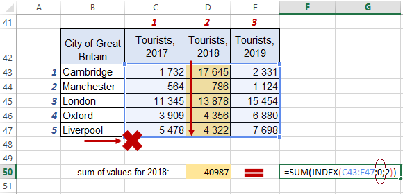
The amount of tourists for 2018 in five cities in the UK is 40,987 people.

Similarly to this scheme, we are looking for an answer to the second point. Only now we need to read the data from the row, so we put zero in place of the column number:

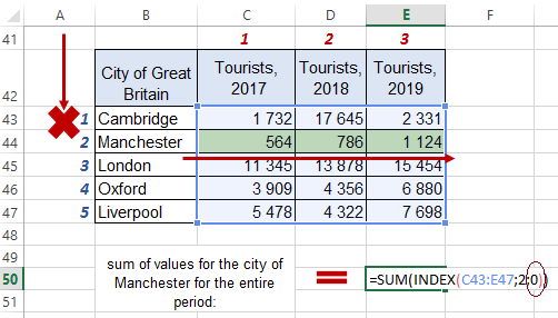
And we get the answer to the second point - in total there were 2,474 visitors in Manchester in three years.

For example, the simplest tasks and solutions of the same type through a function are often used. But in work, the amount of data is always larger and more complex, so more than one function or a combination of them are used to solve such tasks. We will consider such examples below.

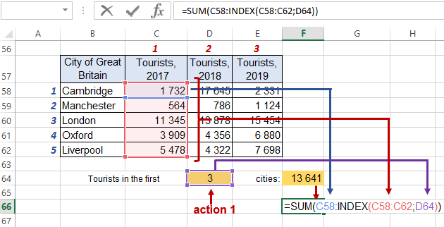
The formulation of the function can be modified depending on the problem statement. Suppose we need to determine and show how many tourists were together in 2017 in the first three cities on the list - Cambridge, Manchester and London. Then we use the SUM function again, but in the place where the end of the range of values on which we are searching is indicated, we insert our INDEX. In simple word, the range for summation looks like this: (beginning: end). The beginning will be the first cell of the array, as usual, and we will replace the end. We will indicate the amount of cities for which we will count people (action 1). Then, when we make function INDEX, we indicate that the first argument is the numerical range of all five cities for the year 2017, and the second is our amount of cities (cell D64):

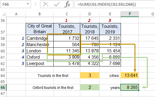
In the same way, you can complete the following task: find the sum of visitors to Oxford for 2017-2018. In this case, we do everything in the same way, only we select the horizontal range C61:E61 :

At the end, it is not necessary to refer to the cell with the written total searched values, you can immediately write the numeric 3 in the first example and the numeric 2 in the second example, everything will work exactly the same:

and

are identical.

Combining several functions can do the same as one single function, but be less demanding on the location of the data, its size or quantity.

Formula INDEX and MATCH is a better replacement for the VLOOKUP function

There are very strong arguments for the advantage of using Excel's INDEX and MATCH formulas over the VLOOKUP function. If you are already familiar with the VLOOKUP function, then you probably know that for it to work correctly, the required data must always be located on the right side of the criteria:

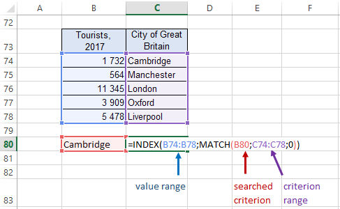
It turns out that in order to work, you first need to arrange the columns in accordance with the requirements, and only then perform actions. But sometimes the very structure of the report or summary that we need to deal with does not allow permutations. Then the INDEX in combination with the MATCH function will come in very handy. INDEX syntax: (array; row_number; column_number). In the first position we will have a range of values (tourists, 2017), instead of the next two we write MATCH (the searched criterion; the range of criteria; 0 (for an exact result)):

Let's consider a more illustrative and real example where you can replace the VLOOKUP. We have two reports: one is about the number of sales of a certain product, and the second is about the price per package of one product. And just the second table has such an arrangement of columns that does not allow us to use VLOOKUP - the values take the first place, and the criteria take the second place:

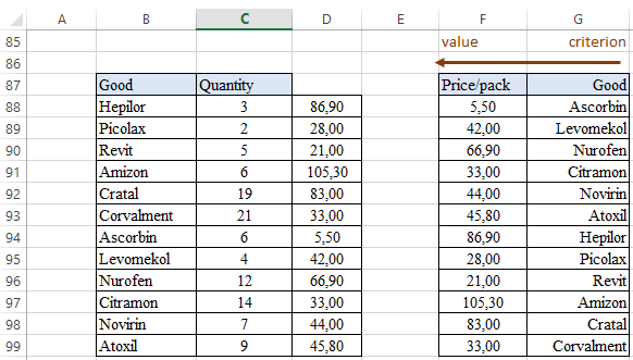
In order to complete the filling of the first table, we do exactly the same as in the previous example - in cell D88 we write INDEX, first of all we indicate the column where the searched values located (price per package). Then we need to indicate where we should look for the values corresponding to the criterion - we adjust the MATCH for our solution: we select the searched criterion (Hepilor), then the array of the searched criteria from the second table:

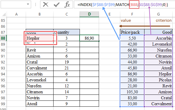
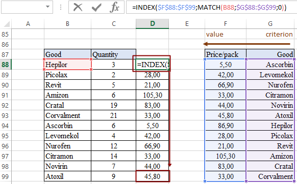
Now we just copy the formula to the end of the column, but do not forget to fix the links, otherwise the array will go down further, and we will get incorrect values. Our table is ready:

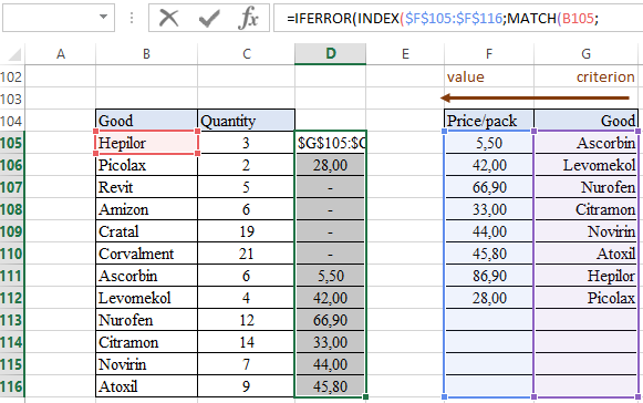
If we do not have data in the second table about price and drugs, we will have a #N/A error in the cell. Now, to our previously used functions, let's add IFERROR, which will help us change the appearance of the report, make it more understandable for the reader. Again, since our second table does not meet the requirements of VLOOKUP, INDEX + MATCH comes to the rescue. We complicate the already existing formula by adding IFERROR, indicating that in the absence of data, we want to see a dash:

download file. Download INDEX and MATCH function examples in Excel

Thus, a formula from a combination of INDEX and MATCH functions works better than the popular VLOOKUP function and has no restrictions for selecting data from a table even for several conditions.