Examples of using the SEARCH function download in Excel
The SEARCH function searches for text, character, number in the specified area. It is similar to the FIND function, which also searches for a value in the specified area, but they have differences, which we will analyze in the examples.
How the SEARCH function works
The syntax for this one is as follows:
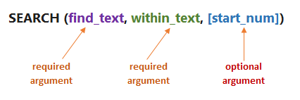
We have the word "Excel". In this example, you need to find the position of the letter "X" in the word. Its will return 2 because the letter is in second place in the searched data:
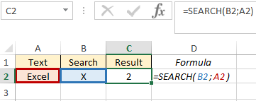
Despite the fact that the searched letter "X" is in uppercase, the function found its counterpart in lowercase and returned the result. This is the difference with the FIND one - it pays attention to the correspondence of registers.
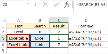
We can also search for a part of a word or a word in the search area, for example, find the word "Excel" in "Exceltable" and "table" in the phrase "Excel table". In the first case, we will get 1 as a result, because the word "Excel" starts with the first character. In the second case, we will have a result of 7, because "table" starts with the seventh character:
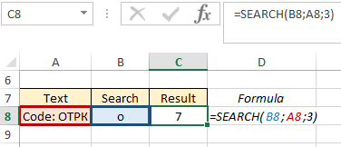
The start_num argument is used when you need to count the position of the character, starting from which the desired value will be returned. For example, you need to track from what position the letter value of the code begins. If you do not specify the position number, we will return the number "2", since the letter "o" in cell A8 is the second in order:
Thanks to this one, it is possible to return parts of phrases that require a condition, and not just a decent character position. To do this, the SEARCH function must be combined with other functions. However, such combinations of functions can be quite voluminous, and there are functions better suited to such tasks.
SEARCH function for a value in an Excel column
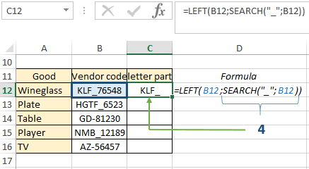
In this example, the formula for combining the SEARCH function with the functions: LEFT, RIGHT, LONG will be used. Let's consider step by step an example where we can extract parts of phrases from the text, from which we will get the desired value. We have a product and a product SKU. Our task is to return only the letter part of the article name. To do this, in cell C12, we begin to write a formula. To get the result, we need the LEFT one.
- The first argument is the text in which the search is performed (cell B12);
- The second argument is the length of the searched word. In the first article, it is equal to 3, and in subsequent articles it changes, so we use the formula SEARCH ("_"; B12).
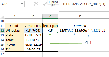
The formula with arguments ("_"; B12) specified that those characters that are located before the underscore character will be returned. Let's check our result:
The SEARCH returned the number 4 (the decent position of the underscore), and as the second argument to the LEFT function, it indicated which characters would be in cell C12. So far, this is not exactly what you need to get - the “_” sign should ideally be absent. Finally, to do this, we will slightly correct the formula: we subtract one before the second argument (the SEARCH formula), by this we indicated that the output of characters will be without an underscore (4-1):
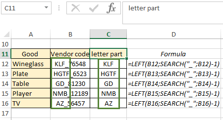
Since our formula is dynamic, we copy it to the end of the column and observe the result of our work - for each article we got a literal value, regardless of the number of letters:
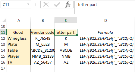
If suddenly you need to change the article in the same table, the function will respond to changes correctly and automatically return the text value of the replaced article. For example, for the product "Wineglass" there will be the letter part "K", for "Plate" - "M", for "Table" - ADCDE:
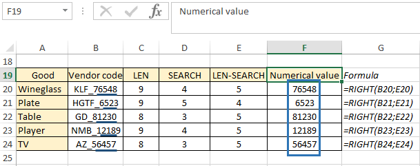
Now let's look at an example where we will extract characters not BEFORE the underscore, but AFTER. The LEN function will help us with this. It helps to find out the length of a text string. In cell C20, write the formula:
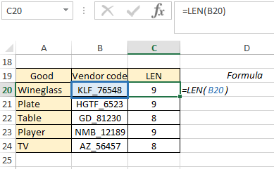
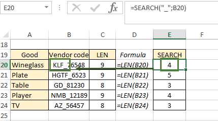
As a result, its returned the length of the product article "Wineglass" to us. Copy the formula to the end of the column and in the next step in cell E20 write the SEARCH formula. The underscore is the value to look up (argument 1), the return value is the position number of the position of the underscore. Copy to the end of the column:
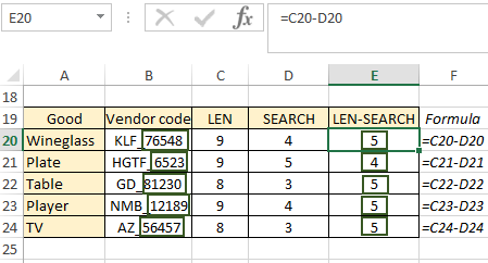
Then we need a column where we subtract the position of the underscore (9 - 4) from the length of the line and copy the formula to the end of the column. That is, this column contains the length of the numeric value of the article (values AFTER the underscore):
Now in cell F20 we write the RIGHT, which will return the text, part of the phrase that we request. The first argument to the formula is the cell that the formula is checking, and the second is the length of the return value:
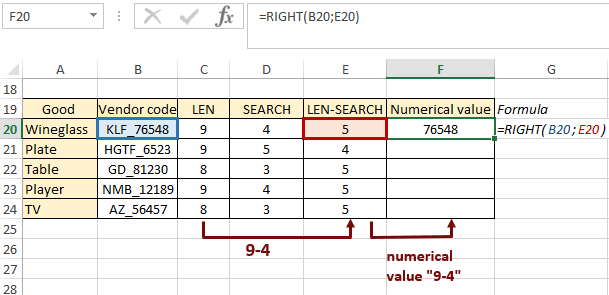
The function returned us the numeric value of the item's SKU. Copy to the end of the column and get the result for each product:
This example was considered in stages for a more understandable algorithm for completing the task, however, you can get a numerical value in one step:
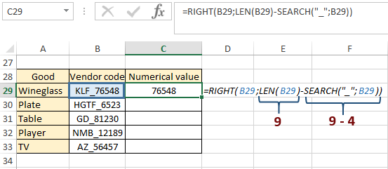
In this example, we did the same thing as before, only we did all the operations in one formula: we found the length of the text, subtracted the length of the text after the “_” sign, and returned this length with the RIGHT.
How to use the SEARCH function with the IF function
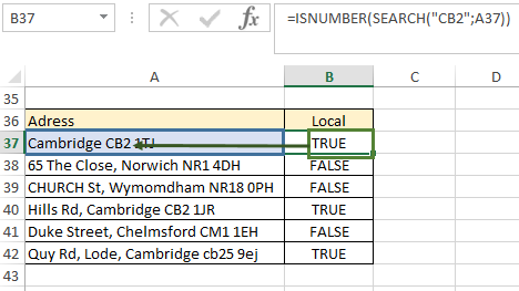
Let's consider an example where we will check the partial match of the text in the checked text. We have several addresses and we need to know if they are local or not:
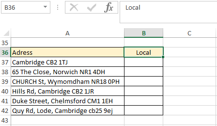
If the postal code starts with CB2, then it is a local address. We can't use the IF in its normal expression because there is a lot of other text in the cells. We need to know if the cell contains the "CB2" part. To better understand the logic of constructing a function, we will do it from a simple to a more complex expression:
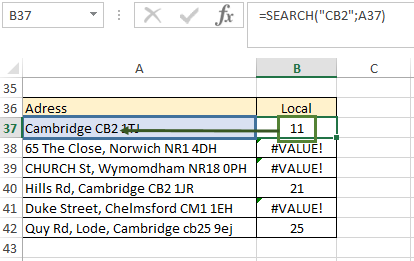
- We build the SEARCH one: 1st argument - "CB2", 2nd argument - cell A37, copy to the end of the column. So we indicated what and where we will look for. Where there is no CB2 text, an error was returned. But now we only have the position number of the text CB2. And the IF function will look for an identical match. That is, it will look for the number 11 in the text of cell A37, which, of course, we will not have anywhere.
- We put the formula of the SEARCH one into the ISNUMBER function (it has only 1 argument), which will be a pointer in the future for IF, that the result of the SEARCH function is a number (as now, we have 11):
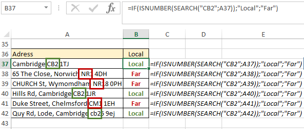
- We put the resulting formula in IF, indicating that for the TRUE value we will have the word "Local", and for the FALSE value - "Far". Copy to the end of the column:
 Download examples of formulas with the SEARCH function in Excel
We now have address information based on their zip code. It's a logical assumption that one could also use FIND, but since FIND is case-sensitive, SEARCH would be more useful and reliable.
