How to use LINEST function in Excel for multiple linear regression
The task of finding a functional relationship is very important, therefore, to solve it, MS Excel introduced a set of functions based on the least squares method. As a result, not only the coefficients of the function that approximates the data are given, but also the statistical characteristics of the results obtained.
Meaning of the output statistical information functions LINEST
LINEST function calculates statistics for a series using the least squares method, calculating a straight line that best approximates the available data. The function returns an array that describes the resulting straight line.
The general syntax of the LINEST function call is as follows:
=LINEST(Knowns_y’s,[Knowns_x’s],[Const],[Stats])
To work with the function, you must fill in at least 1 required and, if necessary, 3 optional arguments:
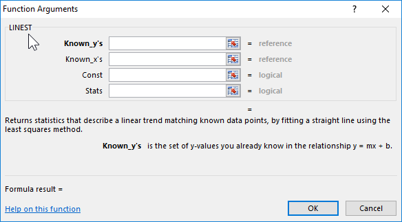
- Knowns_y’s is the set of values of y, which are already known for the relation y = mx + b.
- [Knowns_x’s] is the set of known x values. If this argument is omitted, then it is assumed that this is an array {1,2,3,...} of the same size as known_y.
- [Const] is a logical value that indicates whether the constant b is required to be 0. If in the LINEST function the constant argument is FALSE, then b is set equal to 0 and the values of m are chosen so that the ratio y = mx is satisfied.
- [Stats] is a logical value that indicates whether additional regression statistics are required.
Examples of using LINEST in Excel
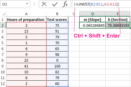
To solve the first problem - the ratio of student preparation hours for a test and test results, like x and y, respectively - the following procedure should be applied (due to LINEST being a function that returns an array):
- Select the range D2:E2, since LINEST returns an array of two values horizontally but not vertically.
- Enter the known values of y - points that students earned on the last test (cell range B2:B12).
- Then enter the known values of x — the number of hours students spent preparing for the tests (range A2:A12).
- Omit the argument [Const].
- Omit the argument [Stats].
- Enter the formula using Ctrl + Shift + Enter.
The result of applying the function becomes:
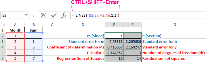
Now, using the example of solving the second task, let's analyze the need for displaying not only the slope and segment, but also additional statistics. For example, on the A1:B6 range, we will build a table with the ratio of y and x corresponding to the amount of money earned by the student for a period of 5 months. Since we have only one variable x, it is necessary to select a range consisting of two columns and five rows. It is important to note that in the event that there are more variables x, the number of columns may vary according to their number, but there will always be 5 rows.
In relation to the problem we are solving, let us select the range E2:F6, then enter the formula similarly to the previous problem, but in this case, the third and fourth arguments will be assigned the value 1 corresponding to TRUE. To display the statistics of the LINEST function, you need to press Ctrl + Shift + Enter, the result should correspond to the following figure, which shows the designation of additional statistics:
Let us return to example number 1, concerning the relationship between hours of preparing students for the test and points for the test. Add to the condition of the problem data on points for homework - representing the additional variable x, which indicates the need for multiple regression.
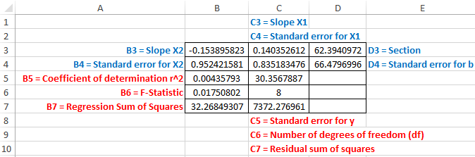
In the case of multiple regression, when the “ y ” values depend on two variables “ x ”, LINEST returns 12 statistics. In the figure with a modified table from example 1, the following notation is used:
- y = dependent variable;
- x1 = independent variable 1 = points for homework;
- x2 = independent variable 2 = test preparation hours.
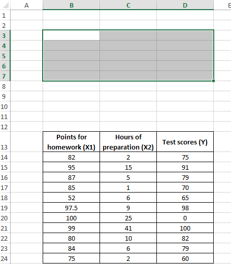
To perform multiple regression:
- Select the range B3:D7 (number of columns = number of variables +1; the number of rows is always 5).
- Type the formula =LINEST(D14:D24,B14:C24,1,1). For the argument [Knowns_x’s], select both columns of x values from the range B14:C24.
- Enter a function using the Ctrl + Shift + Enter keys.
- Note that although the x1 values are in the B14:C24 range to x2, the slope is first indicated for x2.
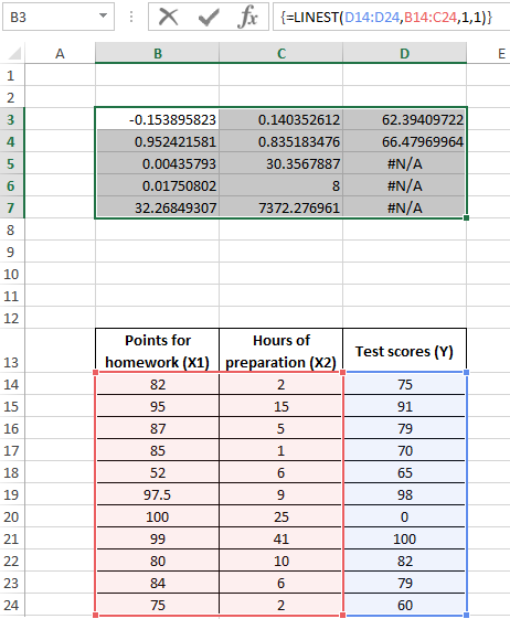
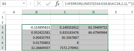
The range D5:D7 contains the error #N/A - meaning that the formula cannot detect the values for these cells. Visually, the presence of an error distracts from the essence of the solution, so further we will propose the option of getting rid of it. So, if we supplement the formula containing LINEST function with IFERROR, then the table can be significantly improved, the result of which is presented below:
The distribution of statistics in the table is presented in the following figure:
Download examples of how to use LINEST in Excel
As a result, we received all the necessary output statistical information that interests us.
