Examples of FREQUENCY in Excel to calculate repetition rates
FREQUENCY function is used to determine the number of occurrences of certain values in a given interval and returns data as an array of values. Using the FREQUENCY function, we will learn how to calculate the frequency in Excel
Example of using the FREQUENCY function in Excel
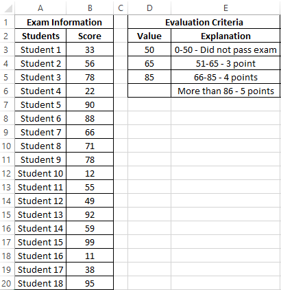
Example 1. Students of one of the groups at the university have passed an exam in physics. When assessing the quality of the exam, a 100-point system is used. To determine the final score on a 5-point system, the following criteria are used:
- From 0 to 50 points - the exam is not passed.
- From 51 to 65 points - a score of 3.
- From 66 to 85 points - score 4.
- Over 86 points - score 5.
For statistics, it is necessary to determine how many students received 5, 4, 3 points and the number of those who failed to pass the exam.
Enter the data in the table:
To solve, select the area of 4 cells and enter the following formula:
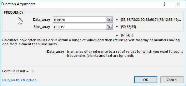
Argument Description:
- B3:B20 is an array of student grades;
- D3:D5 - an array of criteria for finding the frequency of occurrences in the data array of estimates.
Select the range F3:F6, first press the F2 key and then the Ctrl + Shift + Enter key combination so that the FREQUENCY function is performed in the array. Confirmation that everything is done correctly will serve curly brackets {} in the formula bar along the edges. This means that the formula is executed in an array. As a result, we get:
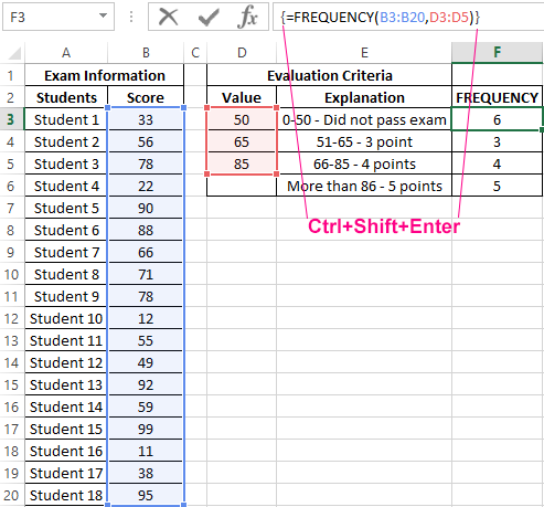
That is, 6 students did not pass the exam, grades 3, 4 and 5 received 3, 4 and 5 students, respectively.
An example of determining the probability using the FREQUENCY function in Excel
Example 2. It is known that if there are only two possible scenarios, the probabilities of the first and second are 0.5, respectively. For example, the probabilities of a “eagle” or “tail” falling on a coin tossed are ½ and ½ (if we neglect the possibility of a coin falling on an edge). A similar calculated probability distribution is typical for the following =RANDBETWEEN(1, 2), which returns a random number in the range from 1 to 2. 20 calculations were performed using this function. Determine the actual probabilities of the occurrence of the numbers 1 and 2, respectively, based on the results obtained.
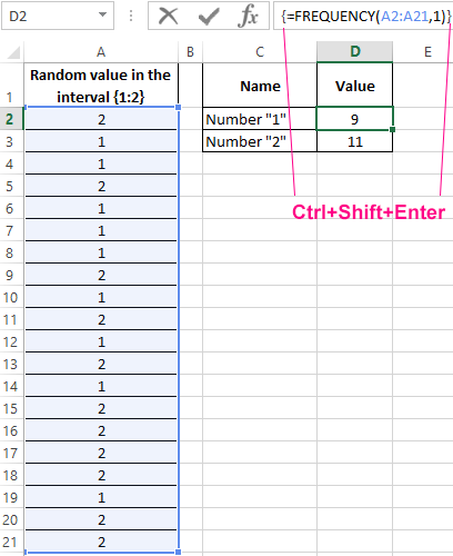
Fill in the source table with random values from 1 to 2:
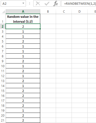
To determine random values in the source table, a special function was used:
=RANDBETWEEN(1,2)
To determine the number of generated 1 and 2 use the formula:
=FREQUENCY(A2:A21,1)
Argument Description:
- A2:A21 - an array of function-generated =RANDBETWEEN(1,2) values;
- 1 - search criteria (the FREQUENCY function searches for values from 0 to 1 inclusive and values> 1).
As a result, we get:
We calculate the probabilities by dividing the number of events of each type by their total number:
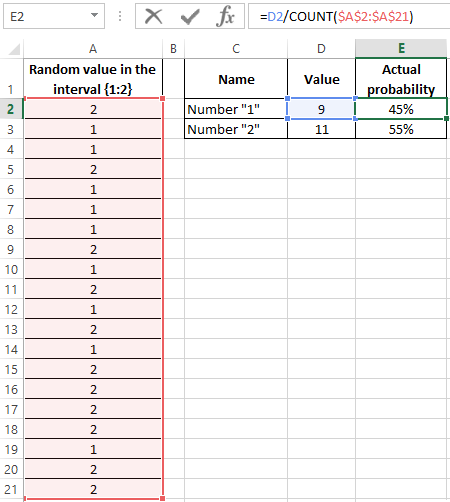
To count the number of events, we use the function =COUNT($A$2:$A$21). Or you can simply divide by the value of 20. If the number of events and the size of the range with random values are not known in advance, then you can use the reference to the whole column in the arguments of the COUNT function: =COUNT(A:A). This automatically calculates the number of numbers in column A.
The probabilities of "1" and "2" are 0.45 and 0.55, respectively. Do not forget to assign the percentage format to the E2: E3 cells to display their values in percents: 45% and 55%.
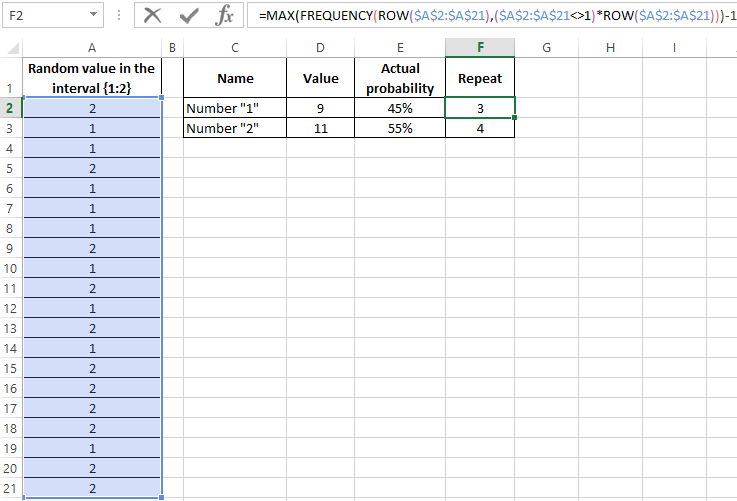
Now we use a more complex formula to calculate the maximum repetition rate:
Formulas in cells F2 and F3 differ only in one number after the comparison operator “not equal”: <> 1 and <> 2.
Interesting fact! Using this formula, you can easily check why the doubling strategy at the casino roulette does not work. This strategy of bet management in gambling is also called Martingale. The fact is that the number of random repetitions in a row can reach 18 times or more, that is, eighteen times in a row red or black. For example, if the rate of $2 to double 18 times - this is more than half a million dollars "drawdown". This is a failure for any risk planning techniques. It should also be borne in mind that, in addition to “black” and “red”, sometimes “zero” also drops out, which finally destroys all the chances. It is also interesting that the sum of all numbers in the roulette from 0 to 36 is 666.
How to calculate non-recurring values in Excel?
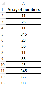
Example 3. Determine the number of unique entries in the array of numeric data, that is, not duplicate values.
Source table:
Determine the desired value using the formula:
In this case, the FREQUENCY function performs a check on the presence of each of the elements of the data array in the same data array (both arguments coincide). Using the IF function, a condition is defined that has the following meaning:
- If the item you are looking for is in a range of values, 1 will be returned instead of the actual number of occurrences;
- If the item is not found, 0 (zero) will be returned.
The resulting value (the number of units) is summarized.
As a result, we get:
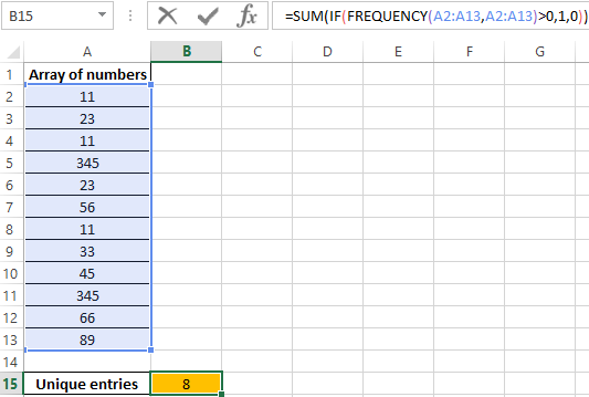
That is, in the specified array contains 8 unique values.
FREQUENCY function in Excel and features of its syntax
This function has the following syntax entry:
=FREQUENCY(Data_array,Bins_array)
Description of the arguments (both are required):
- Data_array - data in the form of an array or a link to the range of values for which you need to determine the frequency.
- Bins_array - data in array format or link is not a set of values into which the values of the first argument of this function are grouped.
Notes 1:
- If an empty array or a reference to a range of empty values was passed as the interval_ array argument, the result of the FREQUENCY function will be the number of elements that enter the range of data that was passed as the first argument.
- When the FREQUENCY function is used as a normal Excel function, a single value will be returned that corresponds to the first occurrence in the interval-array (that is, the first search criteria for the occurrence frequency).
- The array of elements returned by this function contains one element more than the number of elements contained in the array_intervals. This is because the FREQUENCY function also calculates the number of occurrences of values whose values exceed the upper limit of the intervals. For example, in the data set 2.7, 10, 13, 18, 4, 33, 26 it is necessary to find the number of occurrences of values from the ranges from 1 to 10, from 11 to 20, from 21 to 30 and more than 30. The array of intervals should contain only their boundary values, that is, 10, 20, and 30. The function can be written as: = FREQUENCY ({2; 7; 10; 13; 18; 4; 33; 26}; {10; 20; 30}) and the result of its execution will be a column of four cells that contain the following values: 4.2, 1, 1. The last value corresponds to the number of occurrences of numbers> 30 in the dataset.
- If the array_data contains cells that contain empty values or text, they will be skipped by the FREQUENCY function in the calculation process.
Notes 2:
- The function can be used to perform statistical analysis, for example, in order to determine the product names most demanded for buyers.
- This function should be used as an array formula because the data returned to it is in the form of an array. To perform the usual formulas after entering them, you must press the Enter button. In this case, you need to use the key combination Ctrl + Shift + Enter.
Download examples FREQUENCY to calculate repetition rates in Excel
