Excel function for Matrix Multiplication with examples
You can work with a matrix in the Excel just like with a range. That is, a set of adjacent cells occupying a rectangular area.
The matrix address is the upper left and right lower cell of the range indicated by the colon.
Array formulas
Building a matrix of Excel tools in most cases requires the use of appropriate arrays. Their main difference is that the result is not one value but a data set (a range of numbers).
The procedure for applying the data set formula:
- Select the range where the result of the formula action should appear.
- Enter the formula (starting with the sign «=»).
- Press the kea combination Ctrl + Shift + Enter.
The data set formula in curly brackets is displayed in the formula bar.
Select the entire range and perform the appropriate actions to change or delete a data set formula. The same combination is used (Ctrl + Shift + Enter) to enter changes. Part of the data set cannot be changed.
Matrix operations in Excel
You can perform such operations with matrices in Excel as transposition, addition, multiplication by number/array; finding the inverse matrix and its determinant.
Transpose the matrices
Transposing the matrix is an act of changing the rows and columns in places.
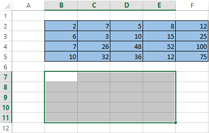
First, note the empty range where we transpose the matrix. There are 4 lines in the original table and the range for the transposition should have 4 columns. For 5 columns there are should be five lines in an empty area, etc.
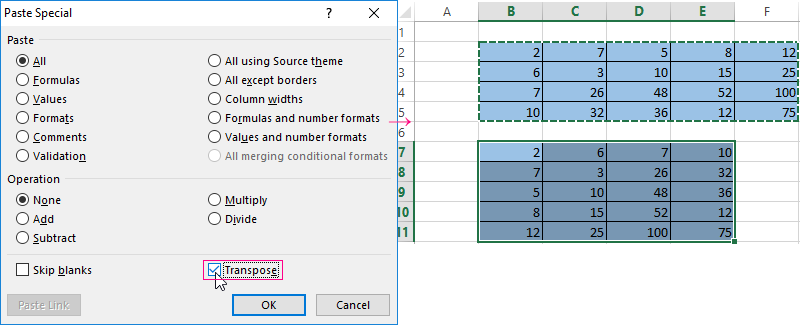
- Method #1. Select the original data array. Click "copy". Select an empty range. Expand the Paste button. Open the "Paste Special" menu (CTRL+ALT+V). Mark «Transpose» operation. Close the dialog by clicking OK.
- Method #2. Select the range B7:E11 with active cell B7 in the upper left corner of the empty range. Select function: «FORMULAS»-«Lookup and Reference»-«TRANSPOSE». The argument is a range with the original array data. Click OK. Now the function produces an error. Select the entire range where you want to transpose the matrix. Press the F2 (go to the formula editing mode). Press the key combination Ctrl + Shift + Enter.
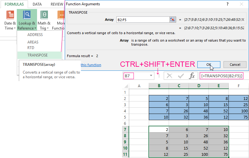
The advantage of the second method: the transposed matrix automatically changes while making changes to the original.
Addition of a matrices
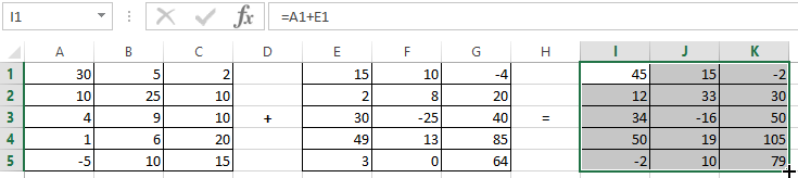
You can sum up matrices with the same number of elements. The number of rows and columns of the first range should be equal to the number of rows and columns of the second range.
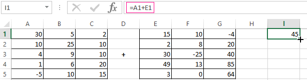
In the first cell of the resulting matrix you need to enter a formula of the next form: = the first element of the first array + the first element of the second: (=A1+E1). Press Enter and stretch the formula to the full range.
Matrices multiplication in Excel
The task is next:
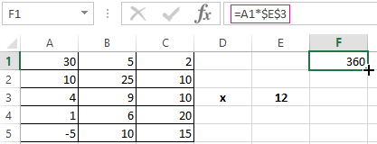
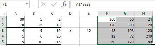
To multiply a matrix by a number you need to multiply each of its elements by this number. The formula in Excel: =A1*$E$3 ( a reference to a cell with a number must be absolute).
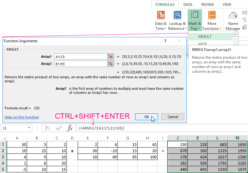
Let’s multiply the matrix with different ranges. It’s possible only to find the product of matrices if the number of columns of the first matrix is equal to the number of rows of the second one.
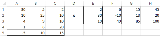
In the resulting matrix, the number of rows is equal to the number of rows of the first array, and the number of columns is equal to the number of columns of the second.
For convenience, we select the range where the multiplication results will be placed. We make the first cell of the resulting field active. Then select: «FORMULAS»-«Math and Trig»-«MMULT» We introduce the formula: = =MMULT(A1:C5,E1:H3). Enter as an array formula (CTRL+SHIFT+Enter).
The inverse matrices in Excel
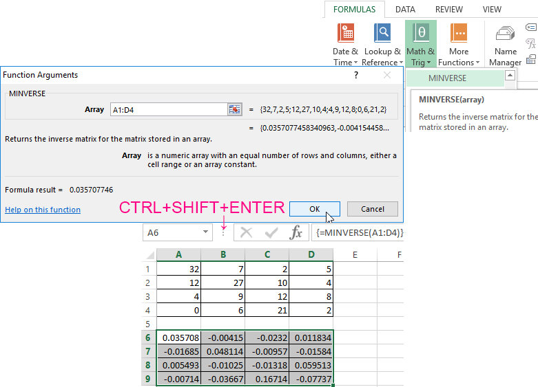
It makes sense to find it if we are dealing with a square matrix (the number of rows and columns is the same).
The dimension of the inverse matrix corresponds to the size of the original. We use: «FORMULAS»-«Math and Trig»-«MINVERSE» function in Excel.
Select the first cell of the empty range for the inverse matrix. We introduce the formula «= MINVERSE(A1:D4)» as a data set function. The only argument is the range with the original. We got the inverse array in Excel:
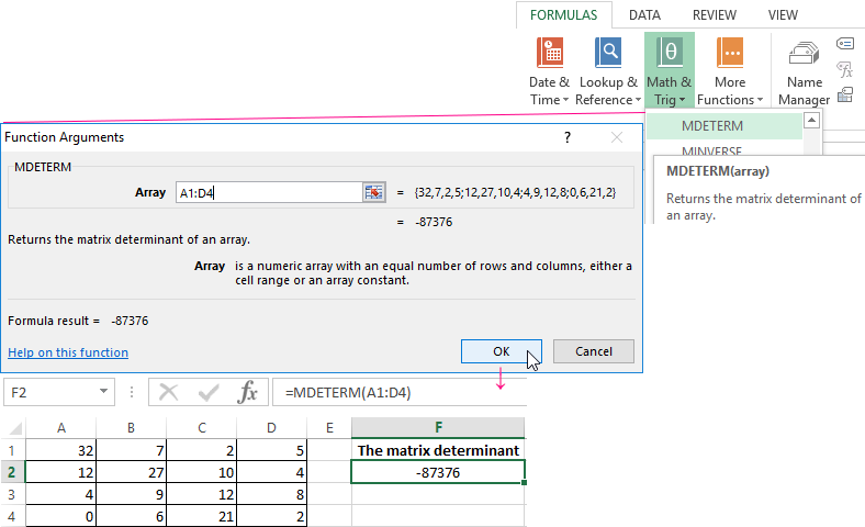
Finding the matrices determinant
This is one single number that is found for a square matrix. We use: «FORMULAS»-«Math and Trig»-«MDETERM» function.
We put the cursor in any cell of the open sheet. Enter the formula: =MOPRED(A1:D4).
Thus, we performed actions with the matrixes using the built-in Excel features.
