The functions of INDEX and MATCH in Excel and examples of their using

There is a very convenient, but for some reason rarely used function in Excel, which is called INDEX. It is convenient because it allows you to output to a value from the range by the given row and column numbers.

In practice, INDEX is rarely used, most likely because of the fact, that these same row and column numbers have to be entered every time. After all, the required value does not always need to be given in order. But then the INDEX function comes to the aid to the function MATCH, which just allows you to find the right position.



The example of using the INDEX and MATCH functions

Let`s consider the interesting example that will allow us to understand the fascination of the INDEX function and the invaluable help of MATCH function. We have the summary table, in which the purchased products are recorded.

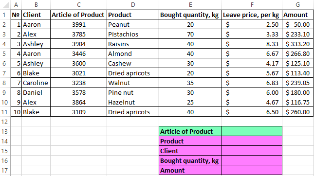
Our goal: to create an order card, where by the article number you can see what kind of product it is, which customer it purchased, how much products were bought and at what total cost. To do this, the INDEX function together with MATCH will help.

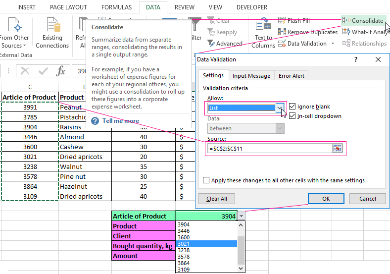
For a start, let`s create the drop-down list for the ARTICLE OF PRODUCT field, so that you do not need to enter numbers from the keyboard, but select ones. To do this, you need to click on the corresponding cell (we have the F13), then to select the DATA - Data Tools - Consolidate. In the window that opens, in the «Allow:» section, select the «List». And as the source, we highlight the column with the articles, including the cap. So we got the drop-down list of articles, that we can choose.

Now you need to do so, that when you select the article, the values in the remaining four lines are automatically displayed. We use the function INDEX. We write it down and study the syntax in parallel.

The array. In this case, this is the entire table of orders. You need to highlight it together with the cap and fixwith the F4 key.

The line number. If we were to withdraw one value, we would write a specific figure. But since we need, so that the result to change, we use the MATCH function. It will look for the necessary position every time we change the article.

We write down the MATCH command and put its arguments.

The desired value. In our case, this is the cell in which the article is indicated the F13. You need to fix it with the F4 key.

The array to be scanned. Because we search for the article, so we highlight to the column of articles together with the cap and to fix the F4.

Type of mapping. Excel offers three types of matching: larger, smaller, and exact match. We have the specific article, so we choose to the exact match. In the program, it is listed as 0 (zero). On this, the arguments for MATCH have ended.

The number of the column. We use the MATCH again. The desired value will be the cell E14, where the name of the parameter we are looking for (PRODUCT) is indicated. The viewed array: the header with names, because the system will search for the word PRODUCT. The matching type: is 0.

Formula:

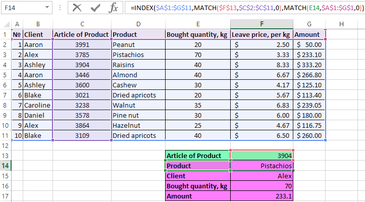
The syntax of the INDEX function is completed. As the result looks like the formula, you can see in the screenshot above. We see, that the article 3516 is really in peanuts. Let`s extend the formula to the remaining rows and check up. Now, changing the article number, we will see who was bought it, amount and how much is.



Search for the index of the maximum number of an array in Excel

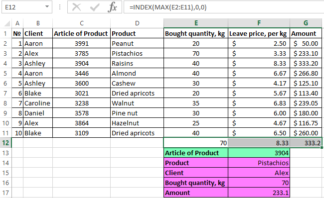
The INDEX function also helps to select to the maximum number from the array. Let`s consider to the same example. We try to determine the maximum values of the purchased quantity of products, prices and amounts.

Let's start with the quantity. In any cell under this column we write = INDEX.

The first argument is not just an array, but the maximum number from the array. Therefore, we additionally use the MAX command and select the corresponding array.

Basically, we don`t need more any arguments, but we need to enter the row and column number. In this case, we write two zeros.

Download example functions INDEX and MATCH

We have obtained the simplest formula, that helps to derive to the maximum value from the array. We will stretch it to the right, having received to the similar information for price and amount.