Examples of formulas with logical functions TRUE FALSE and NOT in Excel
The TRUE function in Excel is intended to indicate a logical true value and returns it as a result of calculations.
The FALSE function in Excel is used to specify a logical false value and returns it accordingly.
The NOT function in Excel returns the opposite of the specified logical value. For example, writing = NOT (TRUE) will return the result FALSE.
Examples of using the logical functions true, false and not in Excel
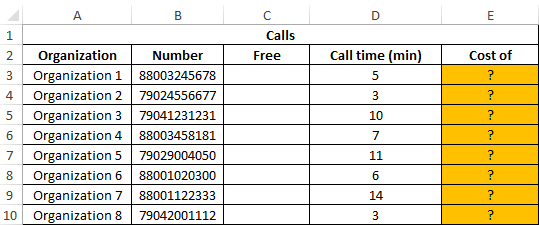
Example 1. The Excel spreadsheet stores the phone numbers of various organizations. Calls to some of them are free of charge (code 8800), while the rest are charged at the rate of 1.5 rubles per minute. Determine the cost of calls made.
Data table:
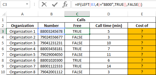
In the “Free” column we display the logical values TRUE or FALSE according to the following condition: is the phone number code equal to “8800”? We introduce the formula in cell C3:
Argument Description:
- LEFT (B3; 4) = "8800" - condition for checking the equality of the first four characters of the string to the specified value ("8800").
- If the condition is met, the TRUE () function will return a true logical value;
- If the condition is not fulfilled, the FALSE () function will return a false logical value.
Similarly, we determine whether the call is free for other rooms. Result:
To calculate the cost, we use the following formula:
Argument Description:
- C3 = TRUE () - checking the condition "is the value stored in cell C3 equal to the value returned by the function (logical truth)?".
- 0- call cost, if the condition is met.
- D3 * 1.5 - the cost of the call, if the condition is not met.
Calculation results:
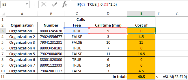
We received the total cost of all calls made by all organizations.
How to calculate the average value of the condition in Excel
Example 2. Determine the average score for the exam for a group of students, in the composition of which there are students who have failed. It is also necessary to obtain an average assessment of performance only for those students who have passed the exam. The grade of the student who did not pass the exam must be counted as 0 (zero) in the formula for the calculation.
Data table:

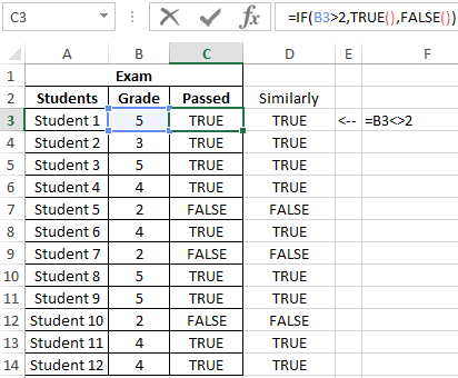
To fill in the “Passed” column, use the formula:
Result of calculations:
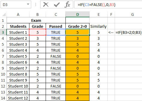
Create a new column in which we rewrite the estimates, provided that grade 2 is interpreted as 0 using the formula:
Result of calculations:
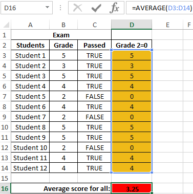
We determine the average score by the formula:
=AVERAGE(D3:D14)
Result:
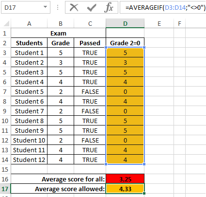
Now we get the average grade point for students who are admitted to the next exams. To do this, we use another logical function AVERAGEIF:
How to get the value module numbers without using the abs function
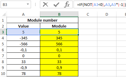
Example 3. Implement an algorithm for determining the value of the modulus of a number (absolute value), that is, an alternative for the ABS function.
Data table:
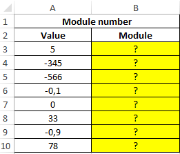
To solve, we use the array formula:
=IF(NOT(A3<0),A3,A3*(-1))
Argument Description:
- NOT (A3: A10 <0) - checking the condition “does the number belong to a range of positive values or is it 0 (zero)?”. Without the use of the function, a longer version of the OR record would not be required (A3: A10 = 0, A3: A10> 0);
- A3: A10 - the returned number (the corresponding element from the range), if the condition is met;
- A3: A10 * (- 1) - the returned number, if the condition is not met (that is, the initial value belongs to the range of negative numbers, to obtain the module, multiply by -1).
Result:
Note: as a rule, the logical values and the functions themselves (TRUE (), FALSE ()) are not explicitly indicated in the expressions, as is done in examples 1 and 2. For example, to avoid intermediate calculations in Example 2, you could use the formula = IF B3 = 2, 0, B3), and also = B3 <> 2.
At the same time, Excel automatically determines the result of calculating the expression B3 <> 2 or B3 = 2, 0, B3 in the arguments of the IF function (logical comparison) and on its basis performs the corresponding action prescribed by the second or third arguments of the IF function.
Features of use of functions true, false, not in Excel
In functions TRUE and FALSE Arguments are absent.
The function does NOT have the following syntax notation:
=NOT( logical value )
Argument Description:
- logical is a required argument characterizing one of two possible values: TRUE or FALSE.
Notes:
- If the argument logical value of the function is NOT used the number 0 or 1, they are automatically converted to logical values FALSE and TRUE, respectively. For example, the function = NOT (0) returns TRUE, = NOT (1) returns FALSE.
- If any numeric value> 0 is used as an argument, the function will NOT return FALSE.
- If the only argument of the function is NOT a text string, the function will return the error code #VALUE !.
- In computing, a special logical data type is used (in programming, it has the name “Boolean” type or Boolean in honor of the famous mathematician George Boole). This data type operates with only two values: 1 and 0 (TRUE, FALSE).
- In Excel, the true logical value also corresponds to the number 1, and the false logical value also corresponds to the numerical value 0 (zero).
- The functions TRUE () and FALSE () can be entered in any cell or used in the formula and will be interpreted as logical values, respectively.
- Both of the above functions are necessary to ensure compatibility with other software products designed for working with tables.
- The function does NOT allow you to expand the capabilities of functions intended to perform a logical test. For example, when using this function as an argument to log_expression of an IF function, you can check several conditions at once.
Download examples of formulas TRUE FALSE and NOT
