Excel IF function with multiple conditions for beginners
One of the most popular and quite easy-to-use IF function is a logical one. It allows you to check some data for compliance with specified conditions and shows the result after comparison.
IF function parameters and how it works in Excel
The syntax of our function in its simplest application is as follows: IF(logical_expression; value_if_true; value_if_false).
Now let's analyze its arguments in more detail:
- Boolean expression - certain data that we have to check for compliance with some of the conditions we have.
- Value_if_true - the result of the check that we will see when the logical expression is true.
- Value_if_false - the result if the condition and our data that we are checking do not match.
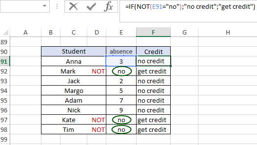
Schematically, it looks like this:
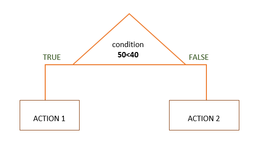
Now let's look at how we can determine the result of the check using the IF. To begin with, we determine WHAT we need to check - the number 50. Then we indicate the condition - “more than 40”, “less than 40”, after which we write the result of the check - “TRUE”, provided that 50 is really more than 40 and “FALSE”, when 50 less than 40. After we have determined what our arguments will look like, we begin to piece together our formula:
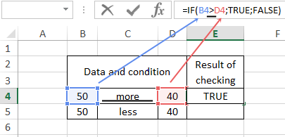
The function tested the expression "50 is greater than 40" and determined that the result is TRUE (cell E4).
We check the following condition in the same way, simply by replacing the “greater than” operator with “less than”:
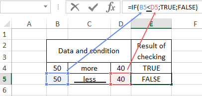
Since 40 is greater than 50, the test determined that our expression is FALSE.
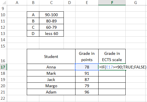
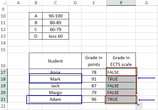
Now let's look at more illustrative examples of using the IF. We have a list of students and grades in points obtained for the exam. We need to find a straight-a student who got a grade greater than or equal to 90. We begin to compose a function, cell F17. The value in cell E17 must be greater than or equal to (>=) 90, then we will get the result "TRUE". When the value in cell E17 is less than 90, the value "FALSE" will be returned:
And we copy the value of the cell to the end of the column, so we found students who got a result greater than or equal to 90 points:
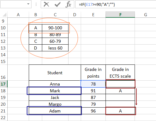
But such table values do not allow the user to correctly read the information that we wanted to convey. Then we need to replace the words TRUE and FALSE with more accepted and understandable ones. Here we will need a table of correspondences of marks on the ECTS scale to marks in points B10:C13. Suppose that with a true result we will have a grade A, which corresponds to scores from 90 to 100, and with a false result, the cells will remain empty, after which we copy the first cell to the end of the column and our table will become more informative:
IF and VLOOKUP formula
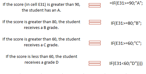
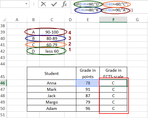
Now let's look at an example of using nested formulas and a situation where they can come in handy. In the previous example, we identified a straight-a student, but we still have blank fields. We also need to determine what letter grade other students will get. We indicate that students with a score greater than or equal to 90 will receive an A grade: =IF(E31>=90; "A"; Then, in place of the "value_if_false" argument, insert the formula IF(E31>=80; "B"; and in place of the argument value_if_false of the same formula, insert another formula IF(E31>=60; "C"; and in place of the third argument of this function we write the last condition, not forgetting to add brackets: IF(E31<60)))):
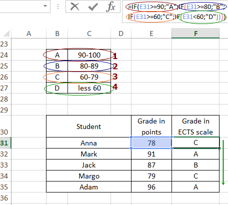
We copy the formula to the end of the column and thus we have built a nested function. However, sometimes when writing such a function, you need to take into account one nuance - it works correctly as long as the data for comparison is specified from a larger value to a smaller one (1,2,3,4):
Here's what happens when we specify the conditions for comparison in reverse - from smallest to largest:
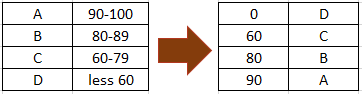
The logic is that the formula, during the check of the first cell, determined that the value is greater than 60 and gave the corresponding result - "C". Further verification did not continue. There are situations where the score instead of A will be A +, A, A-, such a branching will be for each letter and there will be more letter marks themselves. Then the process of creating a nested function will be very long, there will be a lot of nested formulas and it will become easy to get confused. In this case, VLOOKUP can be used instead of IF. First, let's modify our smaller table. Such changes are due to the peculiarities of the work of the VLOOKUP function:
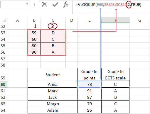
The VLOOKUP formula will look for the approximate value of cell E60 in the range B53:C56 in the second column and pass the found values to the main table:
Function IF multiple conditions
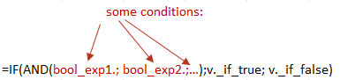
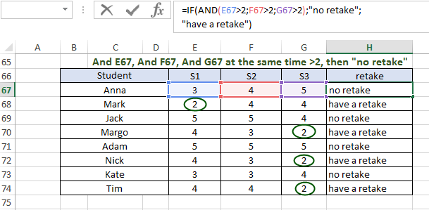
Now let's look at examples where our data must meet several conditions. The IF function together with the AND function has the following syntax:
For example, we have a list of students and data on their grades in three subjects. We need to check if the student has a grade of 2 in at least one subject and indicate if the student has a retake:
In addition to the AND function, you can use the OR one. The difference between them is that when AND is used, all logical expressions must match the condition at the same time. When using the OR formula, it is sufficient that at least one logical expression matches the condition.
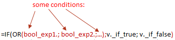
For example, we have a list of students and the condition that if there is at least one grade of 3, the student does not receive a scholarship. We check if the content of the cells in the items is equal to the number 3:
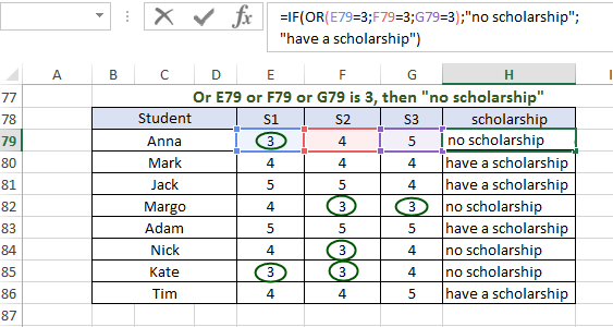
The IF function in combination with the NOT function is very similar in its operation to the simplest example of the IF function with one condition and two results, only now our logical expression will change the condition to the opposite. We have a list of students and information about the availability and number of absenteeism. We need to indicate that in the absence of absenteeism, the student has a credit, and in any other cases - not a credit.
Provided that the value “no” is NOT located in cell E91 (NOT (E91 \u003d “no”)), our result is a pass, in any other case it is not a pass:
There may be a situation when we need not only the results of processing conditions, but also their graphical representation. Besides AND, OR, NOT functions, we can combine IF + MAX. Let's consider a situation where we can use this.
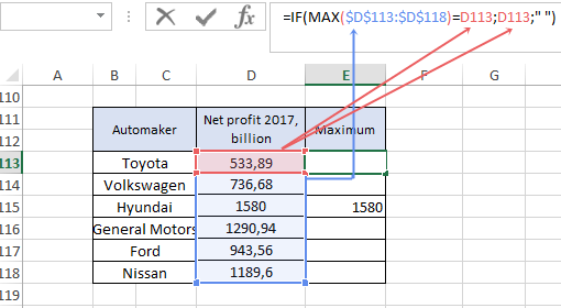
We have a net income statement for several companies. We want to see only the indicator that is the maximum. To do this, we use the MAX function together with the IF function: IF (MAX (specify the range in which we will look for the value) = cell that the function will pass through the range; value if true (checked cell); value if false (do not specify anything)) . In cell E113 we write the formula, do not forget about absolute references for the range D113:E119, otherwise it will shift when copied, copy the formula to the end of the column:
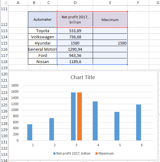
Let's diversify our work results and create a graph that will also highlight our maximum number: select the range D111: E119 - Insert - Recommended charts - Select the first chart and OK. Now we have data presented in tabular and graphical form:
Now the maximum number is highlighted not only in the table, but also in the diagram. But now we have two of these values - from both columns. Let's edit our chart a bit. On the chart, select any of the Series, open the menu by right-clicking on it, select Format Data Series, set Series Overlap to 100% and consider the result we got:
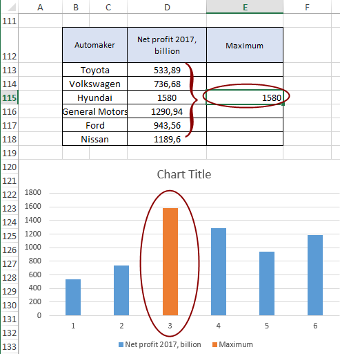
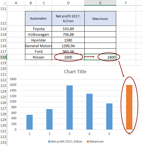
The data from the third column overlapped the data from the second and we got the highlighting of the maximum indicator. Now, when we need to change any number in the second column, our formula will re-detect the maximum number from the "Net Profit" column, show it in the "Maximum
" column, and then we will see it among the other numbers and on the chart automatically. For example, let's say the new number for Nissan is 1600. Here are the changes:
 Download example function if with multiple conditions in Excel
The formula in column E has changed its calculations and these changes are displayed on the graph - the new found maximum number is highlighted. Such processes will occur with any change in the indicators in the "Net profit" column.
