IRR function in Excel and the example how to count IRR
For calculating the internal rate of return (of the internal rate of return, IRR) in Excel the IRR function is used. Its features, syntax, examples we are discussed in this article.
The features and syntax of the IRR functions
One of the methods for evaluating of investment projects – is the internal rate of return. The calculation in automatic mode can be performed with using the =IRR() function in Excel. It finds the internal rate of return for a number of cash flows. The financial indicators should be represented by numerical values.
The amounts inside the flows can fluctuate, but the receipts are regular (every month, quarter or year). This is the required condition for a correct calculation.
The internal rate of return (IRR, internal rate of return) – this is the interest rate of the investment project, in what the present value of cash flows is zero. At this rate, the investor will return the funds originally invested. The investments consist of payments (amounts with the «-» sign) and income (with the «+» sign), which occur in the same length of time intervals.
The arguments of the IRR function in Excel:
The arguments of the IRR function in Excel:
- Values: The values. The range of cells containing the numerical expressions of money. For these amounts, you should to calculate the internal rate of return.
- Guess: The assumption. There is a figure that is supposedly close to the result. The argument is optional.
There are secrets of the function IRR work:
- In the range with money amounts must be contained at least one positive and one negative signification.
- For the IRR function so important the order of payments or receipts. That is, the cash flows should be entered into the table in conformity with the time of their occurrence.
- The texts or logical meaning, empty cells are ignored in the calculation.
- In the Excel program, the iteration (selection) method is used for calculating to the internal rate of return. The formula performs a cyclical calculations from the value that specified in the «Assumption» argument. If the argument is missed, it happens from the value 0. 1 (10%).
When calculating the IRR in Excel, the #NUMBER error may occur. Why? Using the iteration method in the calculation, the function finds the result with the accuracy of 0. 00001%. If after 20 attempts you can not get the result, the IRR will return to the error value.
When the function shows the error #NUMBER!, you need to reiterate the calculation with other meaning of the «Assumption» argument.
The examples of the IRR function in Excel
The calculation of the internal rate of return we consider in the elementary example. There are following input data:
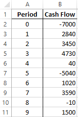
The amount of the initial investment is 7000. During the analyzed period there were two more investments – there are 5040 and 10.
Let`s go in the «Formula» tab. In the category «Financial» we find the IRR function. We fill in these arguments.
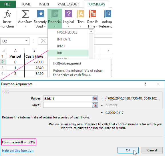
The values – is the range with the sums of cash flows, for which it is necessary to calculate the internal rate of return. We are omitting the assumption now.
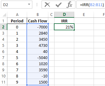
The required IRR (internal rate of return) of the analyzed project – is 0.209040416569432. If we transfer the decimal expression of the value in percentage, then we get the rate of 21%.
In our example, the calculation of the IRR is carried out for annual flows. If you need to find the IRR for monthly flows in just a few years, it's better to enter the «Assumption» argument. The program can not cope with the calculation for 20 attempts – the error #NUMBER! will appear.
One more indicator of the efficiency of the investment project is NPV (the net discounted income). NPV and IRR are linked: the IRR defines the discount rate at which NPV = 0 (that is, the project costs are equal to the revenues).
For calculation NPV in Excel, the =NPV() function is applied. To find the internal rate of return using the graphical method, you need to build the change schedule in NPV. To do this, in the formula for calculating NPV we will substitute to the different values for discount rates.
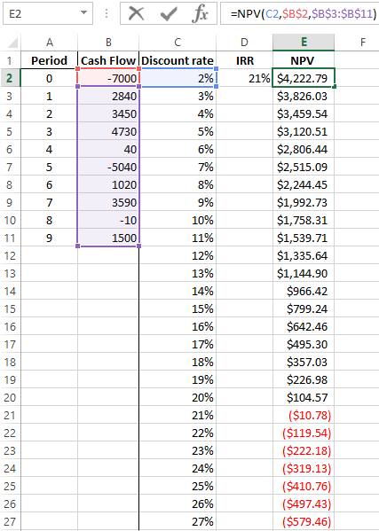
On the grounds of the obtained data, we plot the schedule change in NPV.
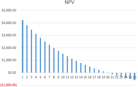
The intersection of the graph with the X axis (when the project's net present value of income is zero) will give us the IRR index for this project. The graphical method showed the result, that is similar to found in Excel.
How to use the IRR indicator:
If the IRR value of the project is higher than the cost of capital for the enterprise, you must accept this investment project.
That is, if the loan rate is less than the internal rate of profitability, then borrowed funds will bring profit. Since in the implementation of the project we will get a higher percentage of income, than the amount of capital will be higher.
Download example IRR and NPV functions count in Excel.
We return to our example now and suppose, that for the launch of the project a loan was taken in the bank at 15% per annum. The calculation showed that the internal rate of return was 20. 9%. You can earn on this project.
