Example MATCH function for finding occurring values in Excel
MATCH function in Excel is used to find an exact match or the closest (less or more than the specified depending on the type of matching specified as an argument) value specified in the array or range of cells and returns the position number of the found element.
Examples of using the MATCH function in Excel
For example, we have a series of numbers from 1 to 10, written in cells B1:B10. Function =MATCH(3,B1,B10,0) will return the number 3, because the desired value is in cell B3, which is the third from the point of reference (cell B1).
This function is convenient for use in cases when it is necessary to return not the value contained in the desired cell, but its coordinate relative to the range in question. If arrays are used for constants, which can be represented as arrays of “key” - “value” elements, the FIND function returns a key value that is not explicitly specified.
For example, the array {"grapes"; "apple"; "pear"; "plum"} contains elements that can be represented as: 1 - "grapes", 2 - "apple", 3 - "pear", 4 - "plum ", Where 1, 2, 3, 4 - the keys, and the names of fruits - values. Then the function =MATCH("apple",{"grapes","apple","pear","plum"},0) returns the value 2, which is the key of the second element. The counting is performed not from 0 (zero), as it is implemented in many programming languages when working with arrays, but from 1.
MATCH function is rarely used independently. It is advisable to use it in conjunction with other functions, for example, INDEX.
Formula for finding inaccurate text matches in Excel
Example 1. Find the position of the first partial match of a string in a range of cells that store text values.
View source data table:
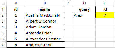
To find the position of a text string in a table, we use the following formula:
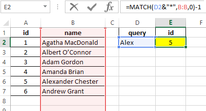
=MATCH(D2&"*",B:B,0)-1
Argument Description:
- D2 & "*" is the sought value consisting of the last name specified in cell B2 and any number of other characters (“*”);
- B:B - reference to the column B: B, in which the search is performed;
- 0 - search for exact match.
A unit is subtracted from the obtained value to match the result with the id of the entry in the table.
Search example:
Comparison of two tables in Excel for the presence of discrepancies
Example 2. Excel stores two tables that appear to be the same at first glance. It was decided to compare one similar column of these tables for the presence of discrepancies. Implement a way to compare two cell ranges.
View of data table:
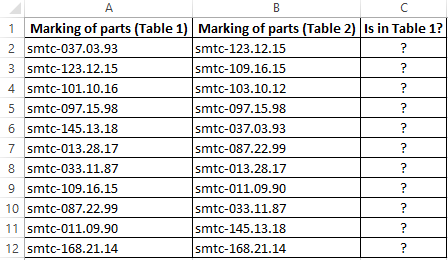
To compare the values in column B:B with the values from column A:A, use the following array formula (CTRL+SHIFT+ENTER):
MATCH function searches for a TRUE logical value in the array of logical values returned by the EXACT function (compares each element of the A2:A12 range with the value stored in cell B2 and returns an array of comparison results). If the MATCH function has found the value TRUE, the position of its first occurrence in the array will be returned. ISNA function will return FALSE if it does not accept the # N / A error value as an argument. In this case, the function IF returns the text string “is”, otherwise - “no”.
To calculate the remaining values, let us “stretch” the formula from cell C2 down to use the autocomplete function. As a result, we get:
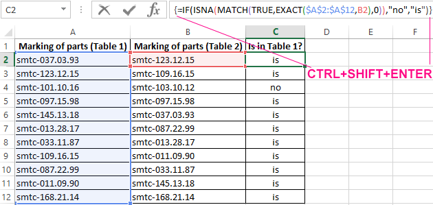
As you can see, the third elements of the lists do not match.
Finding the nearest greater knowledge in the range of Excel numbers
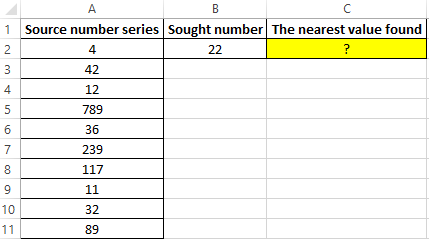
Example 3. Find the nearest smaller number to 22 in the range of numbers stored in an Excel spreadsheet column.
View source data table:
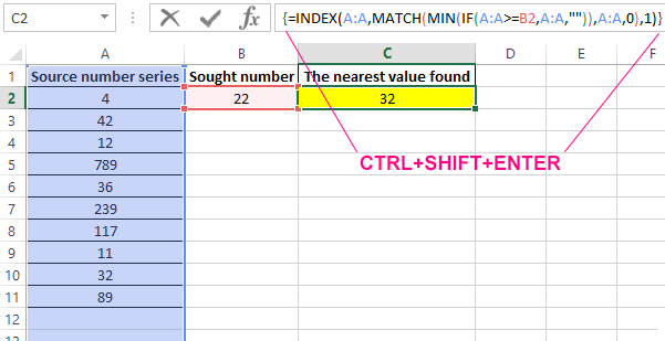
To search for the nearest larger value specified in the entire column A:A (a numerical series can be updated with new values) use the array formula (CTRL + SHIFT + ENTER):
MATCH function returns the position of the element in column A: A, which has the maximum value among the numbers that are greater than the number specified in cell B2. INDEX function returns the value stored in the found cell.
The result of the calculations:
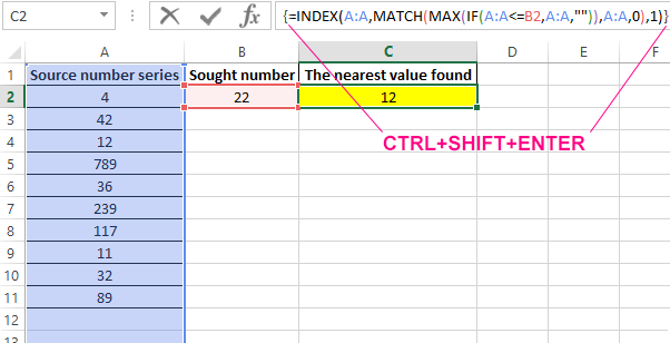
To search for the nearest smaller value, you only need to slightly change this formula and it should also be entered as an array (CTRL + SHIFT + ENTER):
Search results:
Features of using the function MATCH in Excel
The function has the following syntax entry:
=MATCH(Lookup_value,Lookup_array,[Match_type])
Argument Description:
- Lookup_value is a required argument that accepts textual, numeric values, as well as data of a logical and reference type, which is used as a search criterion (for comparing values or finding an exact match);
- Lookup_array is a required argument that accepts data of a reference type (references to a range of cells) or an array constant in which the search for the position of an element is performed according to the criteria specified by the first argument of the function;
- [Match_type] is an optional argument to fill in as a numeric value that defines how to search in a range of cells or an array. It can take the following values:
- -1 - search for the smallest nearest value given by the argument is_value in an ordered or descending array or range of cells.
- 0 - (by default) searches for the first value in an array or range of cells (not necessarily ordered), which is exactly the same as the value passed as the first argument.
- 1 - Search for the largest nearest value given by the first argument in an ordered array of cells in ascending order or range.
Download examples MATCH for finding occurring values in Excel
Notes:
- If a text string was passed as an argument to the Lookup_value, the MATCH function will return the position of the element in the array (if one exists) without case-sensitive characters. For example, the lines "New York" and "new york" are equivalent. To distinguish between registers, you can optionally use EXACT function.
- If the search using the function in question did not return results, the error code #N/A will be returned.
- If the argument [Match_type] is not explicitly specified or takes the number 0, wildcard characters can be used to search for partial match of text values (“?” Is the replacement of any single character, “*” is the replacement of any number of characters).
- If the data object passed as an argument to the Lookup_array contains two or more elements corresponding to the desired value, the position of the first occurrence of such an element will be returned.
