Step-by-step instruction of function LOOKUP in Excel examples

The LOOKUP function is used when it is necessary to find the corresponding value from one column/row in the same position (that is, opposite the value) from another column/row.



Practical operation of the VIEW function in Excel

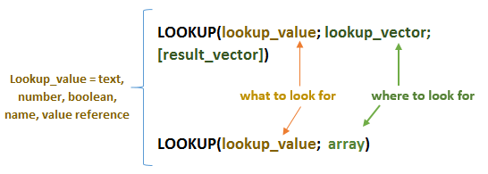
How the LOOKUP function works? The function syntax is as follows:

The first argument, Lookup_Value, can be of any type, depending on the table data and the desired result. The Result_Vector argument is optional and must have the same size as the Lookup_Vector argument. The second variant of the syntax is not used as often and is intended for compatibility with other programs. It is best to use the VLOOKUP function instead of an array. On the first example, let's consider the principle of operation of LOOKUP and all the nuances of the task. We have a table with data on the boundary value of the sound frequency and its characteristics. To begin with, let's perform the simplest task - we need to find a characteristic for a frequency of 100 Hz. We indicate the number "100", then select the range A3: A6, in which the desired value is located. The last step is to specify B3:B6, from which we will return the characteristic:

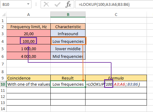
As a result, we got the characteristic "Low frequencies", since this is exactly what is in the same position with the number "100" and a match occurred with one of the values. Now let's check how the formula works when looking for a value that has no matches from the data. For example, let's specify the desired number 2000 among the range:

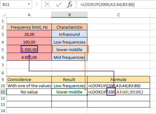
We still got the result. The formula worked as follows - it found the characteristic opposite the value closest to the number "2000" in the direction of decreasing. That is, '2000' falls within the range '1000-4000', but '1000' is less than '4000', so the value corresponding to '1000' is returned. The next step is to select a number greater than the maximum in the "Frequency limit, Hz" column, for example, "5000":

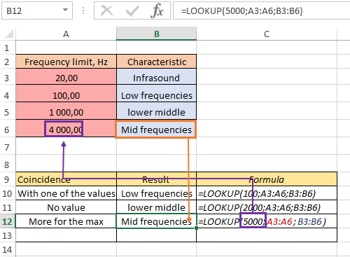
Cell B12 returned "Midrange". The execution logic is very similar to the previous example - the formula rushed to the smallest nearest number and gave the corresponding characteristic. And the last example - we indicate the number that we will be looking for, less than the minimum, for example, "10":

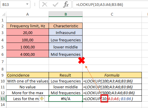
Now we have an error, because there is no number less than "10" in the data, the formula has nothing to rely on, and it returned an error.



How to use the LOOKUP function for different tasks

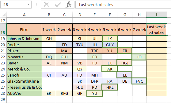
In the following example, we will have a table with sales of firms in different periods. And there will also be weeks in which there were no sales, for example, Roche had no sales on weeks 6 and 7:

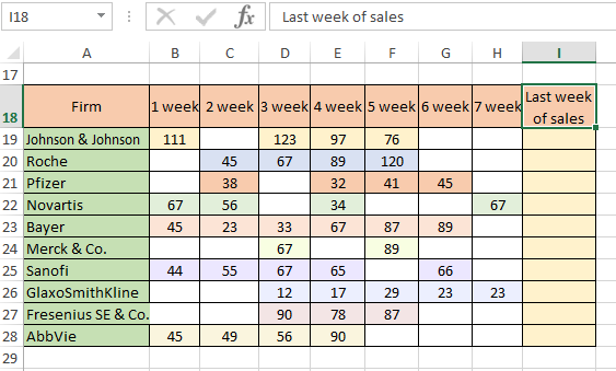
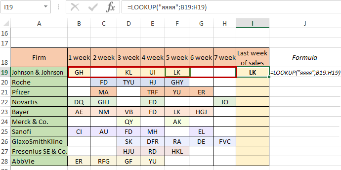
Our task is to extract the latest data for each firm. In the case that the table was completely filled out, the information on fresh sales would always be in the "7 weeks" column. In this example, the work of firms is different. From the table, we can conclude that the last sales of Bayer were in week 6, but there are many companies, and to solve this problem, we will use the LOOKUP function. The value you are looking for must be a number that is greater than any available in the table. It is not necessary to subtract which number will definitely be greater than any of the table, just immediately indicate the value of "9999". Then, for the Lookup_Vector argument, specify the range "B19:H19":

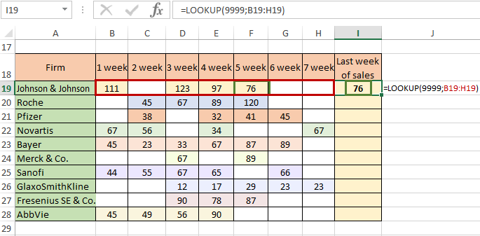
We got the desired value - information about the latest sales, in the 5th week there were sales of 76 conventional units. How the formula works is as follows: LOOKUP looks through the contents of each cell in the range B19:H19, comparing them with the desired value. If the number from the table matched the one we were looking for, the function would return that number. Because the value of each successive cell was not identical, LOOKUP moved from one cell to the next and returned the value of the last cell it checked. Copy the formula to the end of the column and check if we have completed the task:

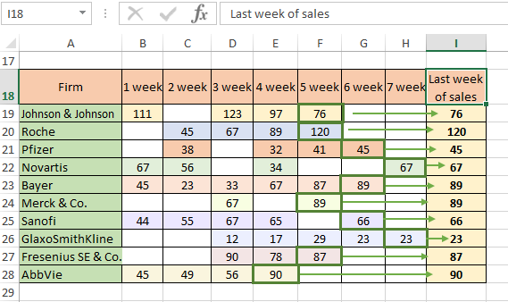
As you can see, for each firm, data on the latest sales was returned. Let instead of numerical values we will have alphabetic ones:

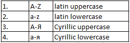
The principle of operation is similar, only now, instead of a very large number, we need to specify a lot of letters - the text “яяяя”. The fact is that the “large” text is a code that consists of letters in the following ascending order:

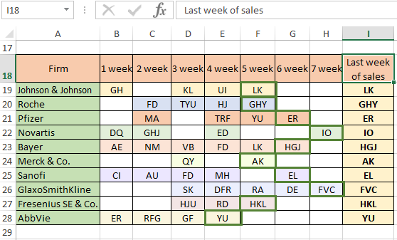
We replace the search text, leave the same range and look at the result:

LOOKUP also worked great for finding the last filled cell in a string. Copy the formula to the end of the column to complete the task:

In the following example, we will make a table with a drop-down list. We have information about companies. We need to create a table in which we will select the company we need from the list and all data on it will automatically be pulled up:

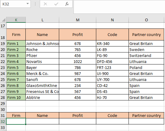
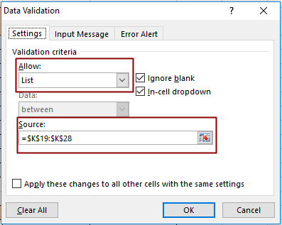
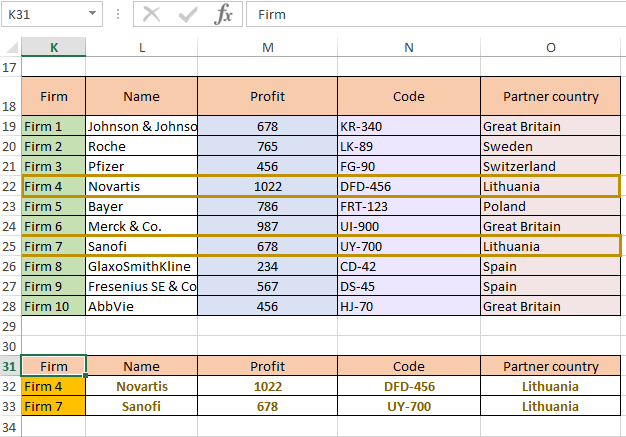
The first step is to create a drop-down list of ten firms. First, make sure that you are on the cell you need (click on cell K32"). Go to the "Data" tab, in the "Data Tools" group, select "Data Validation". A window will appear in which you need to select a list among the “Allow", and specify the range in the "Source". In our case, the range will be a list of ten firms K19:K28:

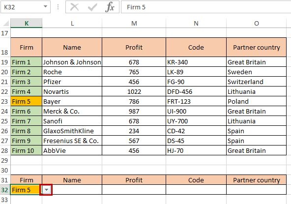
Now a drop-down list pointer should appear near cell K32, thanks to which you can select any of the ten firms:

Now we need to organize automatic pull-up of all data for the selected company. In cell L32 we write the formula LOOKUP. As the desired value, we will have cell K32, since it will change, and depending on these changes, the matches “Firm N = Name” will also change. The second argument will be the range K19:L28, in which the formula will look for matches:

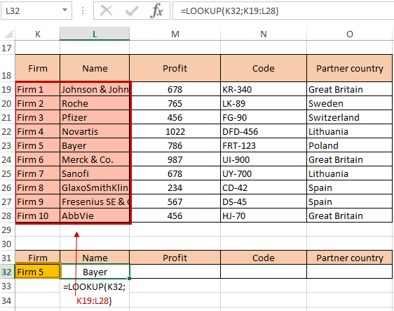
Now we see the result of Bayer, since the first table contains the information that Firm 5 is a firm with the name Bayer. Further, we also build formulas for profit, code, and partner country:

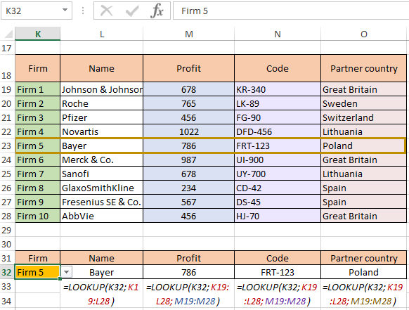
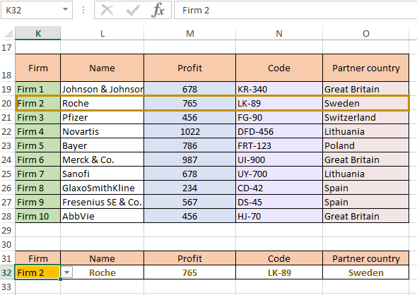
In the formulas where we return data by profit, code, and partner country, the second argument will be divided into two - the viewed vector and the result vector. The first will be unchanged - the range K19:K28, and the second - will change depending on the column from which you want to return data. As you can see, for firm 5 everything worked out correctly - all the elements matched. Now let's choose any other company from the list, for example, 2:

Compare with a glance all the matches. Our table is doing its job. We can also expand the information in the second table a little. Suppose we need to reconcile data for two firms at the same time. To do this, we need to be able to select two firms at once and read their characteristics. First, we copy cell K32 one point down. Near cell K33 there should also be a drop-down list pointer. Then we copy cells L32, M32, N32, O32 in the same way. However, before copying, you need to specify absolute references for the ranges, otherwise the formula will move down one position and we will have errors:

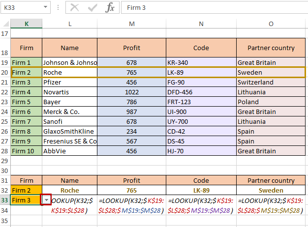
Now we make a copy and we have two rows with drop-down lists of companies and information about them. Let's choose firm 4 and firm 7:

Download step-by-step examples of using the VIEW function in Excel

Our table is complete. You can add characteristics, the number of firms in both tables, it all depends on what task is waiting to be completed.