Example of the function SUMIF for summation in Excel by condition
SUMIF function is used to calculate the sum of the numeric values contained in a range of cells, taking into account the criteria specified as one of the arguments, and returns the corresponding numeric value. This feature is an alternative to sharing SUM and IF functions. Its use allows us to simplify the formulas, since the criterion by which values are summed is provided for directly in its syntax.
Examples of using the SUMIF function in Excel
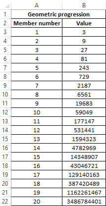
Example 1. The Excel spreadsheet contains members of a geometric progression. What percentage (percentage) is the sum of the first 15 members of the progression of the total amount of its members.
View source data table:
Perform the calculation using the following formula:
Argument Description:
- A3:A22 - range of cells containing sequence numbers of members of the progression, relative to which the summation criterion is set;
- "<=15" is a logical expression that is a summation criterion;
- B3:B22 - the range of cells containing the values of the members of the progression.
The result:
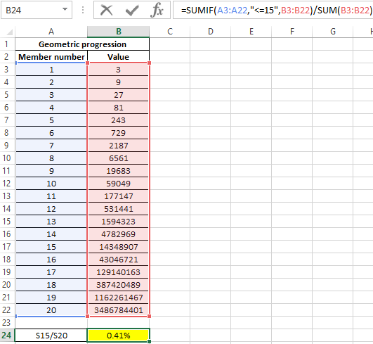
The percentage of the first 15 values (75% of the number of all 20 values) of this geometric progression is only 0.41%.
Sum of cells with a specific value in Excel
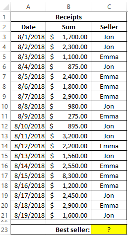
Example 2. Excel spreadsheet shows data on the work of two sellers of a small store. Determine which employee brought more income in 19 working days).
The source table is as follows:
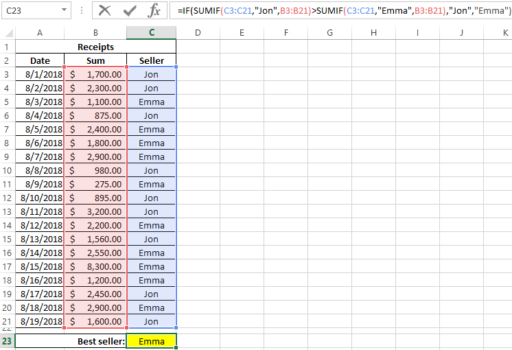
For the calculation we use the function in the formula:
The IF function checks the returned values with the SUMIF functions with the test conditions “Jon” and “Emma”, respectively, and returns a text string with the seller’s last name, the total profit of which was greater.
As a result, we obtain the following value:
How to Excel to sum cells only with a specific value
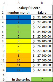
Example 3. The table shows data on the salary of an employee during the 12 months of last year. Calculate employee income for the spring months.
View of data table:
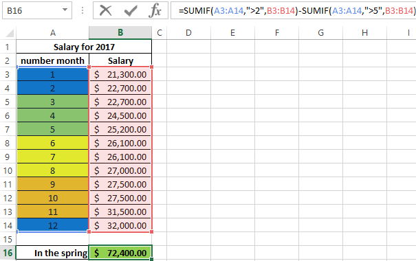
Spring months are the months with numbers 3, 4 and 5. For the calculation we use the formula:
The amount of salaries from the 6th to the 12th month is a subset of the set of the amount of salaries from the 3rd to the 12th month. The difference of these amounts is the desired value - the amount of salaries for the spring months:
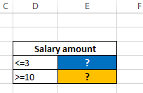
You can use the SUMIF function if you want to define several values at once for different criteria. For example, to calculate the amount of salaries for the first three and three last months of the year, respectively, we make the following table:
For calculations, we use the following formula:
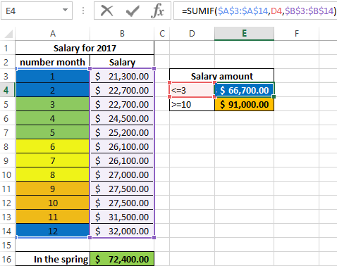
As a result, we get:

Features of using the SUMIF function in Excel
SUMIF function has the following syntax:
=SUMIF(Range,Criteria,[Sum_range]]
Argument Description:
- Range – A required argument that accepts a reference to a range of cells with data for which a particular criterion applies. The cells of this range can contain names, text strings, data of reference type, numeric values, logical TRUE or FALSE, and dates in Excel format. If this range is also a summation range (the third argument is omitted), the final result is not affected by empty cells and cells containing text data.
- Criteria – a required argument that can be specified as a number, text string, logical expression, or the result of a function. The value or expression passed as a given argument is a summation criterion for the function in question.
- [Sum_range] – is an optional argument that accepts a reference to a range of cells containing numeric values for which the sum will be calculated based on the summation criterion (condition).
Notes:
- If the third optional argument is not explicitly specified, the range of cells specified as the first argument is also the summation range.
- The conditions presented in the form of a text string or expression containing the characters “>”, “<”, “=” must be indicated in quotes. If the condition argument is represented as a number, no quotes are required.
- If the condition argument is specified as a text string, you can use a hard criterion (an exact match with the specified substring) or search for values with an inaccurate match, replacing the missing characters with an asterisk “*” (any number of characters) or a question mark “?” (One character).
- If functions refer to cells containing error codes #VALUE! or text strings longer than 255 characters, the SUMIF function may return an incorrect result.
- Arguments can refer to ranges with different numbers of cells. The SUMIF function calculates the sum of values for such a number of cells from the summation range, which corresponds to the number of cells contained in the range. The calculation is performed from the top left cell of the summation range.
- The SUMIF function allows you to use only one summation criterion. If you need to specify several criteria at once, you should use the SUMIFS function.
- The summation criterion does not have to belong to the summation range. For example, to calculate the total salary of an employee for a year, you can enter the formula =SUMIF(A1:A100,”Jon”,B1:B100) in a table that contains data on the salaries of all employees:
Download examples SUMIF for summation by condition in Excel
- a. A1:A100 - a range of cells in which the names of employees are stored;
- b. "Jon" - search criteria (employee name) for the A1 range: A100;
- c. B1:B100 - the range of cells in which data on the salaries of employees are stored (summation range).
