Assigning of SUMIF use function in Excel download for examples
SUMIF is a mathematical function that sums the numeric values in the specified data range by matching them against a specified condition.
Practical work of the SUMIF function in Excel
How does the mathematical and at the same time logical function SUMIF work? Its syntax looks like this:
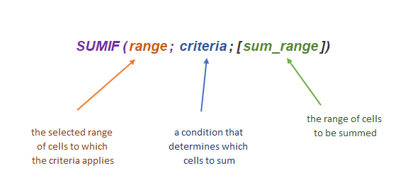
The third argument "Sum_Range" is optional. If it is not specified, the formula will count the cells specified in the first argument. Now, using an example, consider the principle of operation of SUMIF. We have a table with product types of different companies and their revenue. The first task will be to calculate the revenue of Sanofi. To do this, we need to specify the range A3:A11 as the first argument, and specify the condition as the second argument - the Sanofi company. You can enter a text value in the formula, or you can specify a cell reference with a written condition. Then apply the third argument, since the numeric values are in the "Revenue" column - the range "С3:С11":
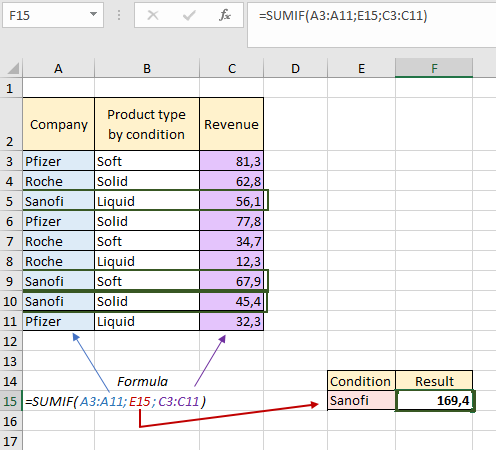
As a result, the formula summed up those numerical values that correspond to Sanofi. The next task will be to find out the amount of revenue of all companies except Sanofi. The “not equal” operator will help us with this. To implement such a query, you need to apply the “<>” operator, the “&” ampersand (for concatenation) and a cell reference with a condition for exclusion to argument 2:
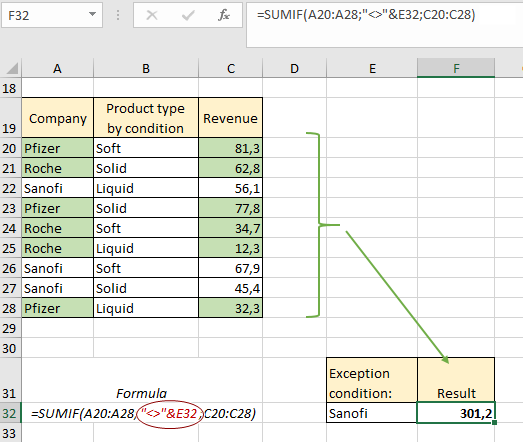
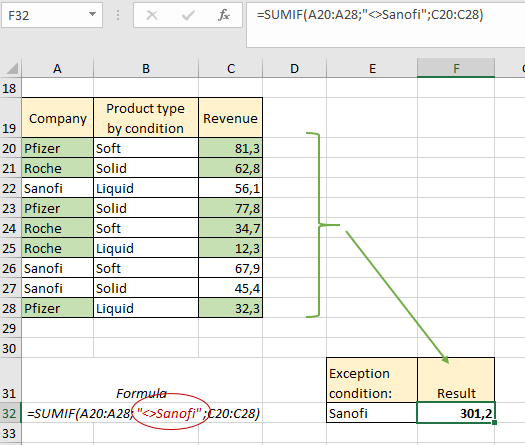
If you use a text value, the ampersand is not needed, then you need to quote both the operator and the text:
Using wildcards in a SUMIF formula
SUMMIF can also be used with wildcard characters such as asterisk and question mark. For example, our companies are divided according to the direction of sales - "Europe" and "Asia". We need to sum the revenue from sales in Europe. To do this, in the “Condition” argument, specify the text we need, place asterisks (wildcard) on both sides, then wrap it in quotes, otherwise the formula will not work:
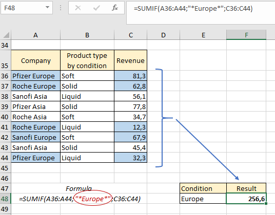
SUMIF summed up only the revenue that companies in Europe received, while all companies were taken into account. That is, we indicated that it doesn’t matter to us what text is still in the cell (at the beginning, middle or end), the main thing is that there is a match for the word “Europe”. If you want to refer to a cell rather than using a text value, then the formula would look like this:
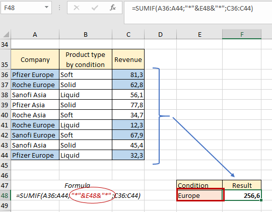
We write ampersands on both sides, connecting the cell with wildcards. If you need to calculate the revenue of those companies in which the word "Europe" is at the end or at the beginning, you need to change the position of the wildcard to the appropriate:
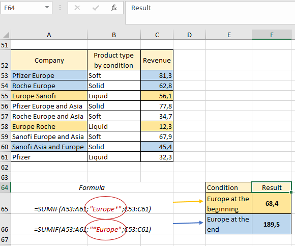
The first formula will work with those companies whose names begin with the word "Europe" (yellow). The second formula will work with those companies whose names end with the word "Europe" (blue color). You can also use the wildcard "?" specify the condition "a word of 6 letters". In the formula, the number of question marks is equal to the number of characters in the word:
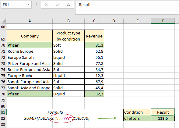
SUMIF went through column A, found those companies that match the condition "??????", that is, 6 letters in the text.
SUMIF function with multiple conditions
Our next task will be to find the proceeds from the sale of ointments and powder preparations. Now we have several conditions at once. Having learned the previous lessons, we can complete this task using two formulas separately, then add them together:
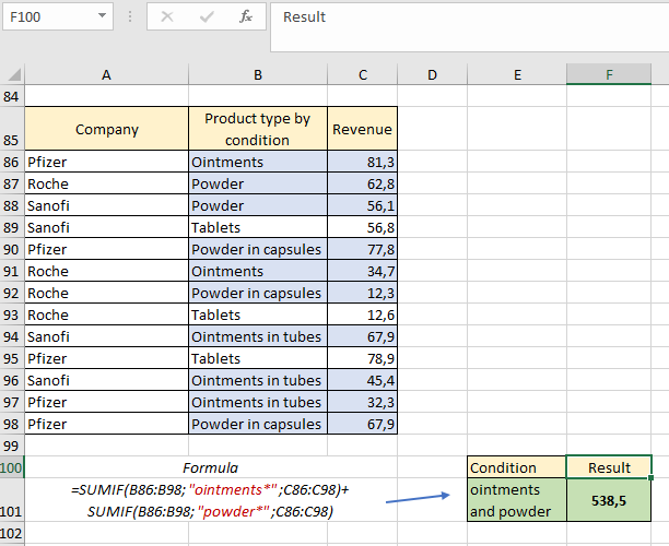
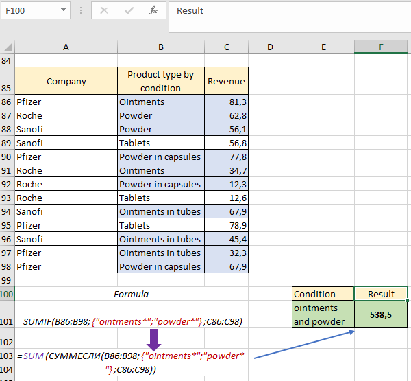
In order for the formula to pull up not only ointments, but also ointments in tubes, we used a wildcard character. The same was done with powders. Then we added the two formulas and got the desired result. However, this simplest method works when there are few criteria. After all, if criteria are added, it will take a very long time to constantly build new formulas. In this case, an array of criteria will help us. As the second argument, we immediately indicate "ointments *" and "powder *" using curly brackets. Then we need to put the constructed formula into the SUM function so that it calculates the contents of our data array:
Practical use of the SUMIF and SUMPRODUCT formulas
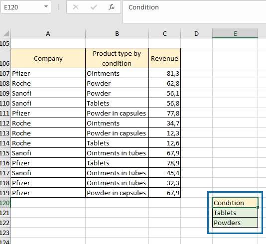
In the following example, we will allocate a separate table for the criteria. For example, we want to search by type "Pills" and "Powder":
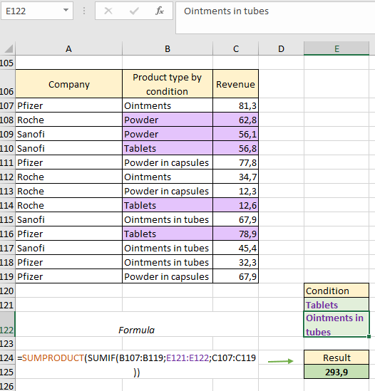
Here we can additionally use the SUMPRODUCT function, which will multiply the elements in the specified arrays and return the sum of these products. As the second argument for the SUMIF function, specify the range of criteria E121:E122. Then we put the whole formula into the SUMPRODUCT function:
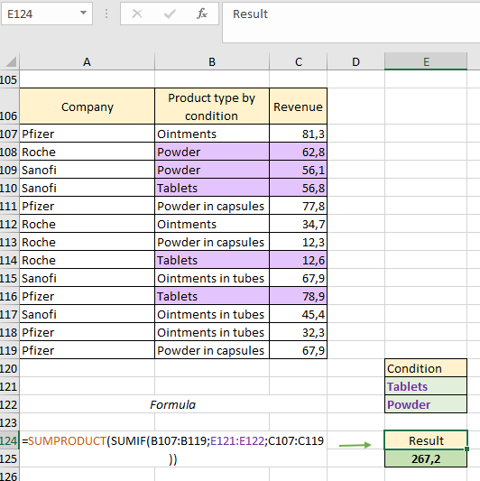
Thanks to the additional table, our formula is dynamic, we can, for example, change the second criterion to “Ointments in tubes” and the formula will recalculate our result:
Example of SUMIF and VLOOKUP formula
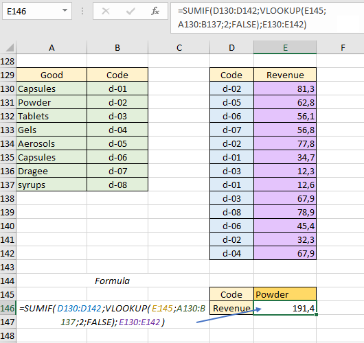
In the following example, we use the SUMIF function in combination with the VLOOKUP function. Let's say we have two tables: the first contains information about the product name and the corresponding code, the second contains information about revenue by product code:
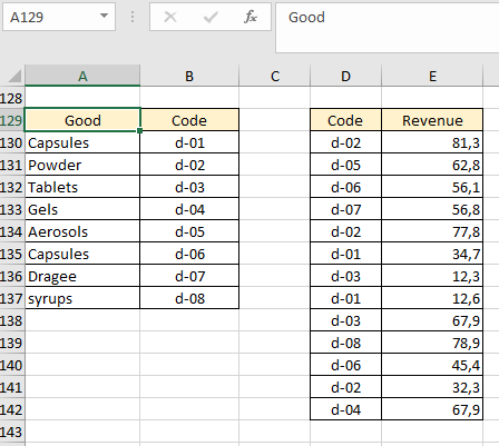
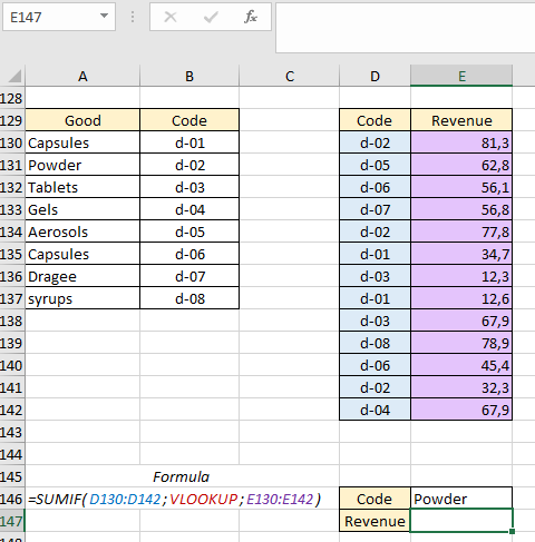
We need to find the amount of revenue for a particular product. In this example, we have a difficulty in that the second table contains several revenue items for one code at once, and it is not possible to add a column with names to the second plate. Let the result of our work be the amount of revenue for the product "Powder". Let's define the first argument for the SUMIF function. Since we are searching by product code, we specify the range from the second table "D130:D142". The second argument will be the VLOOKUP function, which will set the condition. And the third argument will be the range over which the summation takes place - E130: E142:
Now let's look at the VLOOKUP formula. Its syntax is as follows: (lookup value; search range; number of column in return range; return approximate or exact match). The first argument will be cell E147, which contains the product value. The second argument will be the first table A130:B137. The third argument will be the number of the column by which the value will be returned. We also specify the fourth argument "FALSE" for an exact match:
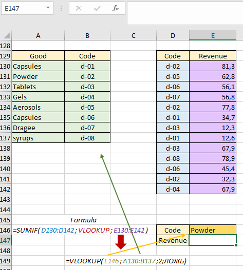
Now we add our formulas into one and get the amount of revenue for the product "Powder":
 Download Practical Examples of SUMIF Function in Excel
The VLOOKUP function retrieved the value d-02 from the table, which corresponded to the searched "Powder". SUMIF then added up all the values in the Revenue column that matched the code d-02, since that value was the summing condition.
