How to Use the Text Functions in Excel with Examples
For the convenience of working with text in Excel, there are text functions. They make it easy to process hundreds of lines at once. Let's consider some of them on examples.
Examples with TEXT function in Excel
This function converts numbers to string in Excel. Syntax: value (numeric or reference to a cell with a formula that gives a number as a result); Format (to display the number in the form of text).
The most useful feature of the TEXT function is the formatting of numeric data for merging with text data. Excel "doesn’t understand" how to display numbers without using the function. The program just converts them to a basic format.
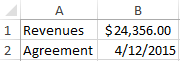
Let's see an example. Let's say you need to combine text in string with numeric values:
Using an ampersand without a function TEXT produces an inadequate result:
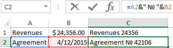
Excel returned the sequence number for the date and the general format instead of the monetary. The TEXT function is used to avoid this. It formats the values according to the user's request.
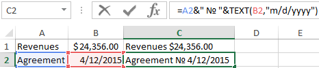
The formula "for a date" now looks like this:
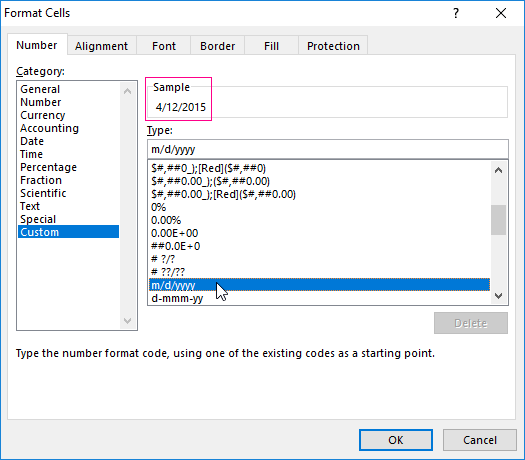
The second argument to the function is the format. Where to take the format line? Right-click on the cell with the value. Click on "Format Cells". In the opened window select "Custom". Copy the required "Type:" in the line. We paste the copied value in the formula.
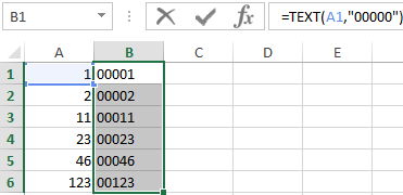
Let's consider another example where this function can be useful. Add zeros at the beginning of the number. Excel will delete them if you enter it manually. Therefore, we introduce the formula:
If you want to return the old numeric values (without zeros), then use the "--" operator:
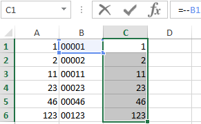
Note that the values are now displayed in numerical format.
Text splitting function in Excel
Individual functions and their combinations allow you to distribute words from one cell to separate cells:
- LEFT (Text, number of characters) displays the specified number of characters from the beginning of the cell;
- RIGHT (Text, number of characters) returns a specified number of characters from the end of the cell;
- SEARCH (Search text, range to search, start position) shows the position of the first occurrence of the searched character or line while viewing from left to right.
The line takes into account the position of each character when dividing the text. Spaces show the beginning or the end of the name you are looking for.
We will split the name, surname and patronymic name into different columns using the functions.
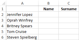
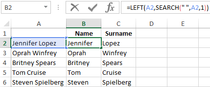
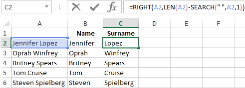
The first line contains only the first and last names separated by a space. Formula for retrieving the name:
The function SEARCH is used to determine the second argument of the LEFT function (the number of characters). It finds a space in cell A2 starting from the left.
For a name, we use the same formula:
Excel determines the number of characters for the RIGHT function using the SEARCH function. The LEN function "counts" the total length of the text. Then the number of characters up to the first space (found by SEARCH) is subtracted.
The formula for extracting the surname:
Next formulas for extracting the surname is a bit different:
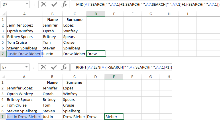
These are five signs on the right. Embedded SEARCH functions search for the second and third spaces in a string. SEARCH ("";A7;1) finds the first space on the left (before the patronymic name). Add one (+1) to the result. We get the position with which we will search for the second space.
Part of the formula SEARCH(" ";A7;SEARCH(" ";A7;1)+1) finds the second space. This will be the final position of the patronymic.
Then the number of characters from the beginning of the line to the second space is subtracted from the total length of the line. The result is the number of characters to the right that you need to return.
Function for merging text in Excel
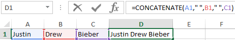
Use the ampersand (&) operator or the CONCATENATE function to combine values from several cells into one line.
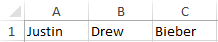
For example, the values are located in different columns (cells):
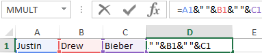
Put the cursor in the cell where the combined three values will be. Enter "=". Select the first cell and click on the keyboard "&" sign. Then enter the space character enclosed in quotation marks (" "). Enter again "&". Therefore, sequentially connect cells with symbols and spaces.
We get the combined values in one cell:
Using the CONCATENATE function:
You can add any sign or string to the final expression using quotation marks in the formula.
Text SEARCH function in Excel
The SEARCH function returns the starting position of the searched text (not case sensitive). For example:
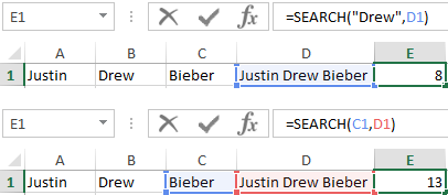
The SEARCH returned to position 8 because the word "Drew" begins with the tenth character in the line. Where can this be useful?
The SEARCH function determines the position of the character in the string line. And the MID function returns symbols values (see the example above). Alternatively, you can replace the found text with the REPLACE.
Download example TEXT functions
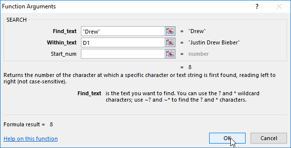
The syntax of the SEARCH function:
- "Find_text" is what you need to find;
- "Withing_text" is where to look;
- "Start_num" is from which position to start searching (by default it is 1).
Use the FIND if you need to take into account the case (lower and upper).
