How to use SUMIFS function to summarize data in Excel
In versions of Excel 2007 and higher, the SUMIFS function works. This function allows you to take several values into account when finding the amount. In the title of the function there is laid it`s purpose: the sum of the data, if there are many of conditions coincides.
The syntax of the SUMIFS and common faults
The arguments of the function SUMIFS:
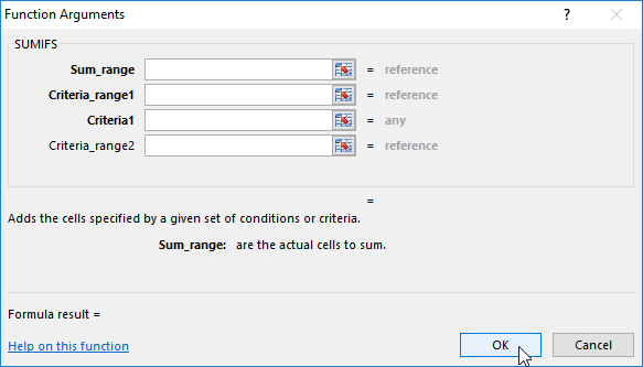
- Sum_range: The range of the cells for finding to the sum. There is required argument, where the data for the summation are indicated.
- Criteria_range1: The range of cells to check the condition: 1. The mandatory argument to which the specified search condition is applied. The data which found in this array are summed within the range for summation (of the first argument).
- Criteria1: The condition 1. There is the required argument that makes up the pair for previous one. This is the criterion by which the cells are determined for summation in the range of the condition 1. The condition can have a numeric format or texts one; it «perceives» to the mathematical operators. For example, is 45; «<100»; «tables», etc.
- Criteria_range2: The range of cells for checking the condition 2; the condition 2; ... dispensable arguments for assigning additional ranges and its conditions. Excel can handle up to 127 arrays and criteria.
There are possible errors at the SUMIFS function:
- The result is 0 (which is the error). This happens when defining conditions in text format. The text must be enclosed in quotation marks.
- The incorrect summation result is returned. If in the range for finding the sum of the cell the value TRUE is contained, then the function returns the result 1. FALSE - 0.
- The function does not work correctly if the number of rows and columns in the ranges for checking conditions does not match which the number of rows and columns in the range for summation.
There are bonuses when using the SUMIFS function:
- The ability of the using wildcard characters when specifying arguments, that allows by an user to find similar but not identical values.
- You can use to the relational operators (<,>, =, etc.).
The examples of the SUMIFS function in Excel
There are the table with the data about the provision of services to clients from different cities with the contract numbers.
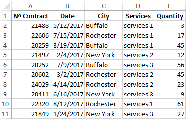
Let`s suppose we need to calculate to the number of services in a certain city with taking into account the type of service. How to use the SUMIFS function in Excel:
- You need to call the «Insert Function » (keys SHIFT+F3). In the «Math & Trig» category we find SUMIFS. You can put the equal sign in the cell and start typing the name of the function. Excel will show a list of functions that have in the name such title. We select the required function by double-clicking of the mouse or simply move to the cursor by arrow on the keyboard down to the list and press the TAB key.
- In our example there is the summation range is the range of cells with the number of services provided. As the first argument you need to choose the «Quantity» (Е2:Е11) column. The name of the column does not need to be included.
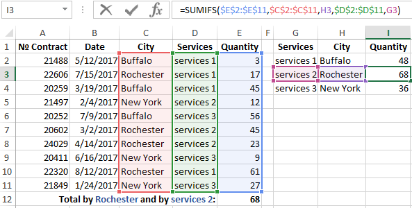
- The first condition that must be met when finding the amount – is a certain city. The range of cells for checking condition 1 – is the column with names of cities (С2:С11). The condition 1 – is the name of the city for which you need to sum up the services. Let's say is «Rochester». The condition 1 – is the reference to a cell with a name of a city (C3).
- For the accounting of the services` type, we set the second range of conditions - the «Service» column (D2:D11). The condition 2 – is the reference to a particular service. In particular, is the service 2 (D5).
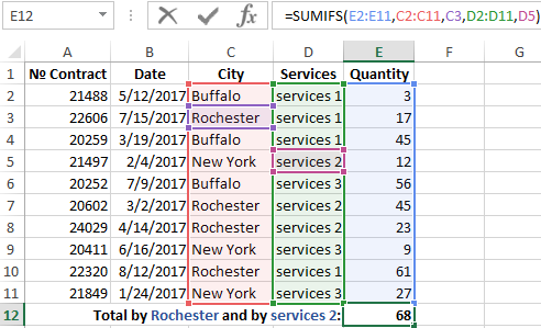
- Here is the formula with two conditions for summation:
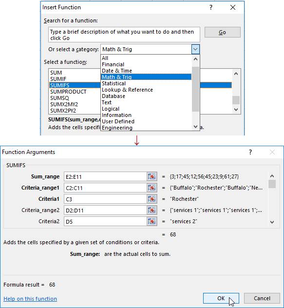
The result of the calculation is 68:
It is much more convenient for this example to make the drop-down list for cities:
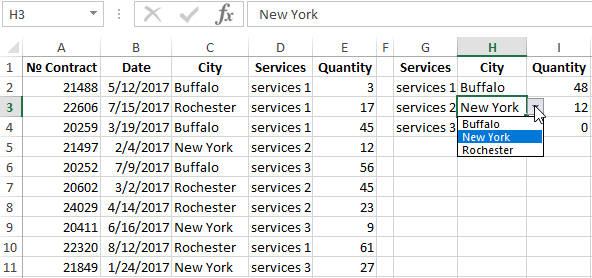
Now you can see how many services 2 are rendered in this city or that one (and not just in Rochester). The formula is slightly modified:
All ranges for summation and checking conditions must be fixed (the button F4). The condition 1 – the name of city – the link to the first cell of the drop-down list. The link to the condition 2 we also made constant. For check from the list of cities we choose «Rochester»:
Download examples using SUMIFS function in Excel.
The result is the same – 68. By the same principle, you can make to the drop-down list for services.
