VLOOKUP function in Excel with step by step examples download

The VLOOKUP function can be used to search for a value by row in a table in a specific dataset. The syntax of it is as follows:

VLOOKUP (lookup value; search range; input value column number; 0 (FALSE) or 1 (TRUE))

FALSE is an exact data, TRUE is an approximate data.

The simplest task for the VLOOKUP function. For example, we have a list of medicines. Our first task is to find the price of Hepilor.

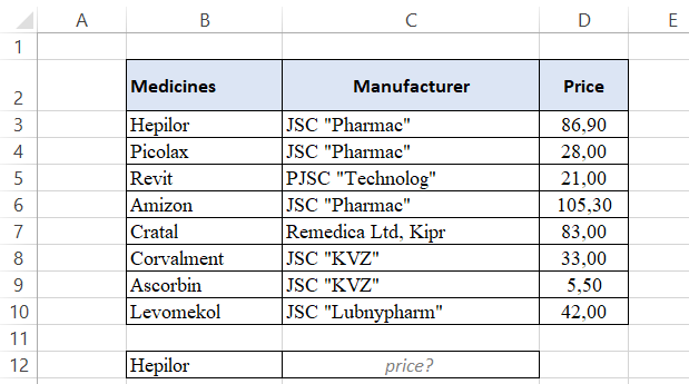
In cell C12, we start writing our formula:

B12 - since we need Hepilor, we select the cell with the pre-written name of the medicines we are looking for.
Next, select the data range B3:D10, where will the search for the numbers we need. The leftmost column of the range must contain the desired criterion by which the numbers is searched.
The next step is to indicate the number of the column in the array B3:D10, from which the information on the same line with Hepilor will be read. The columns are numbered from left to right in the range itself, in our example the first column is B, but not A, since A lies outside the range area.

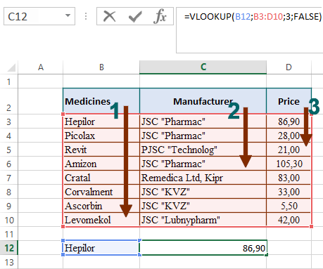
The search in the "Manufacturer" column will work in exactly the same way, you just need to specify the column sequence where the information we need is located - we replace the number "3" in the formula (cell C27) with the number "2":

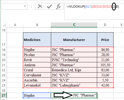
There is a certain feature associated with columns. Sometimes in an Excel file in tables, some cells are merged. In the picture below, in the formula, instead of the serial number of the column, we have the number “3”, but the result is the name of the manufacturer, not the price, as in the first example:

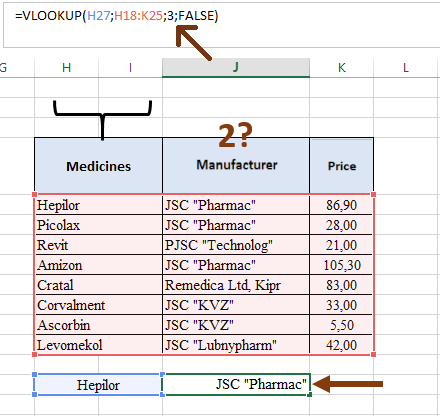
There was a shift in the numbering of the columns just because of the presence of a merging of cells in the "Medicines" column: we combined the "H" and "I" columns, visually the "Medicines" column is the first column, and "Manufacturer" is the second, BUT the formula number them like this:

H – the first;
I – the second;
J – the third;
K – the fourth.

Using the VLOOKUP to search by criteria in this example seems not entirely appropriate, because any product information can be read immediately without searching, but when the range contains hundreds, thousands of names, the one will significantly speed up the process and save a lot of time compared to an independent search.

Using VLOOKUP to work with multiple tables and other functions

In the following example, let's look at how else we can use the VLOOKUP to search and retrieve information by criteria and combine the function with the IFERROR. For example, we have two reports - a report on the quantity of goods and a report on the price per unit of goods, which we need to calculate the cost. Again, with a small amount of data, this can be done manually, but when we have a large amount, its will help us deal with this faster and more efficiently. In cell D3, we start writing the formula:

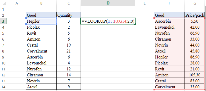
B3 – criterion by which we search for data.
F3:G14 – the range over which our function will search for a match between the criterion and the string data.
The number "2" - the number of the column with the information we need according to the criterion.
The number "0" (or you can use the word "FALSE") - for the accuracy of the results.

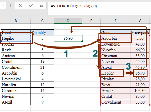
Thus, when we give the formula a search criterion, it starts searching for matches from the top cell of the first column (step 1 in the picture). The one then "reads" all the criteria from top to bottom until it finds an exact match (step 2). When the VLOOKUP reaches Hepilor, it will count the required number of columns to the right (step 3) and give us the desired value for the criterion - the price of 86.90 (step 4):

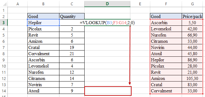
But now we have data only for the first criterion. In order to fill the third column D of the first table to the end, you just need to copy the function to the last criterion. However, at this stage, for correct operation, the range where the search is performed must be fixed, otherwise the data array will “slide” down and we will not succeed. To do this, we use absolute references for the range in cell D3 - select the range F3:G14 with the cursor and press the F4 key, after which we copy the formula to the end of the table:

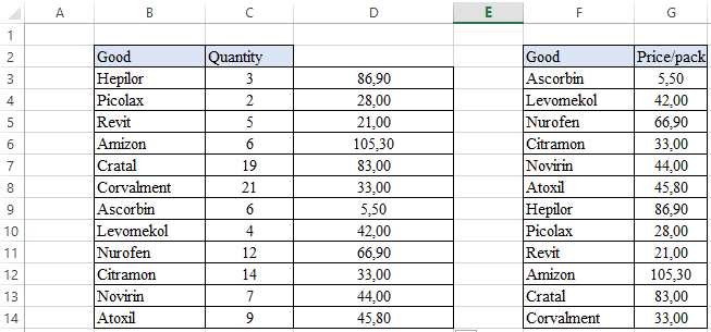
Finally, we get the result we need:

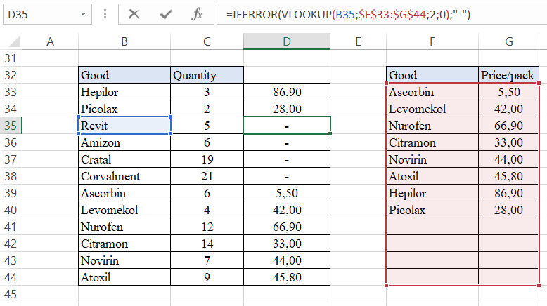
However, our example was based on the full compliance of the criteria from both tables - the same number of goods, the same names. But what if, for example, the last four items were removed from the pack price report? Then we will have a #N/A error in the first table in those positions that are on the same line as the desired criterion:

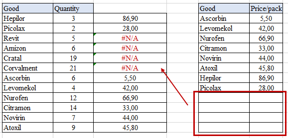
If you are not satisfied with this cell content, you can change table view. To do this, we combine the VLOOKUP function with the IFERROR. The syntax of the last one (value, value_if_error), so the first one will be our used VLOOKUP, and the second one will be what we want to see instead of #N/A, for example, a dash, but necessarily quoted:

As a result, we will get a beautifully designed table with the proper look:

Using an approximate value

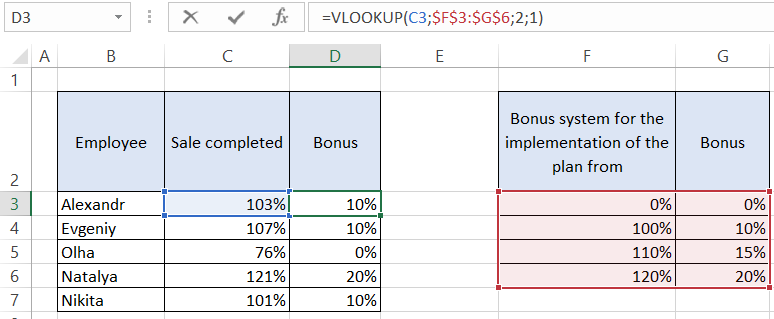
Not always the criterion by which the search takes place must match exactly in the tables. Sometimes a certain range will be enough, which will include the desired criterion. For example, we have a list of employees with their sales plan performance indicators and a motivation system that shows us how many percent of the bonus from the salary the employees earned:

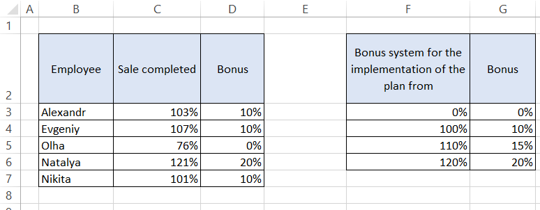
As you can see, the size of the bonus depends on the range according to the bonus system, where the sales performance indicator of a particular employee falls. We see that if the plan is fulfilled by less than 100%, no bonus is awarded, and if by 107% (above 100%, but less than 110%), then the employee receives a bonus of 10%. We need to enter the described bonus indicators using the VLOOKUP function in the “Bonus” column of the first table, only this time the criterion will be in a certain range.

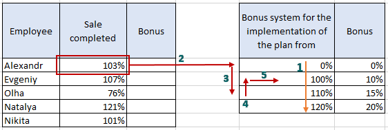
To work correctly, you need to make sure that the range boundaries in the second table of the leftmost column are placed in ascending order from top to bottom (step 1). The formula takes the criterion we have chosen and searches the first column of the second table (step 2), going through all the data from top to bottom (step 3). As soon as the function finds the first value that exceeds the criterion from the first table, it "steps back" (step 4) and reads the value that matches the found criterion (step 5). In other words, with an inexact search, the VLOOKUP looks for a smaller number for the desired criterion:

Thus, our function will look like this:

After that the result of using the VLOOKUP function with an approximate search has this result:

download file. Download all step-by-step examples of VLOOKUP functions in Excel

For example, employee Olga has a bonus of 0%, since she completed 76% of sales, that is, she exceeded the plan by 0%. In addition employee Natalia made sales 21% above the norm and was rewarded by 20%, which we can see if we compare the data from the two tables on our own.

The application of the VLOOKUP function does not end with these examples, there are many other tasks that it is convenient to handle with this one. It makes it easier to work with a large amount of data, minimizes errors compared to independent calculations, and is easy to understand and use.