Working with functions in Excel on examples
The Excel functions – there are computing tools, suitable for various industries: finance, statistics, banking, accounting, engineering and design, analysis of research data, etc.
Merely a scanty part of the possibilities of computational functions are comprised in this tutorial with Excel lessons. We`ll consider the practical application of functions on simple instances & further.
The function of calculating the average number
How to calculate the arithmetic mean in Excel? Make the table, as depicted in the picture:
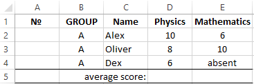
In the cells D5 and E5 we introduce the functions, that help to receive the average of the grades of achievement in the lessons of English & Mathematics. The cell E4 does not matter, so the result will be calculated from 2 estimates.
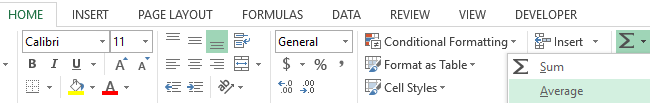
- Work with the cell D5.
- Choose the tool from the drop-down list: «Home» – «Sum» – «Average». In this drop-down list there are frequently used mathematical functions.
- The span is determined mechanically, it remains only to press Enter.
- The function, that includes the cell D5 now, you need to replicate in the cell E5.
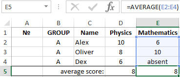
The secondary function in Excel: = AVERAGE () in the cell E5 ignores the text. It will ignore the empty cell also. But if the cell has a value of 0, then the result will change naturally.
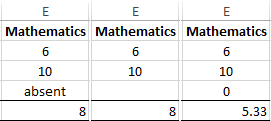
In Excel, there is still the function = AVERAGEA() – the average meaning is an arithmetic number. It differs from the previous one in that:
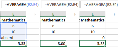
- = AVERAGE() – there are skips cells that don`t contain numbers;
- = AVERAGEA() – there are skips only empty cells, and accepts text values as 0.
The function of counting the number of values in Excel
- In the cells D6 and E6 in our table you need to enter the function of counting the number of numerical values. The function will allow us to learn the number of grades given.
- Go to the cell D6 and pick out the tool from the drop-down list: «Home» – «Sum» – «Number».
- This time, the automatic detection of a range of cells is not suitable for us, so you need to fix it to D2:D4. Press Enter after that.
- From D6 to the cell E6, you should copy = COUNT () – it need for counting the number of non-empty cells.
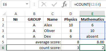
In this example it's clear, that the function = COUNT() overlooks cells, that don`t comprise number or are empty.
The IF function in Excel
In the cells D7 and E7 you need to introduce a logical function, that will allow us to check whether all students have grades. There is example of IF function:
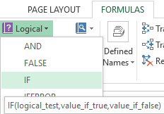
- Go to the cell D7, select the tool: «FORMULAS» – «Logical» – «IF».
- Fill in the arguments of the function in the dialog box, as you can see in the figure and click OK (note, that the 2-nd link $A$4 is absolute):
- The function from D7 is copied to E7.
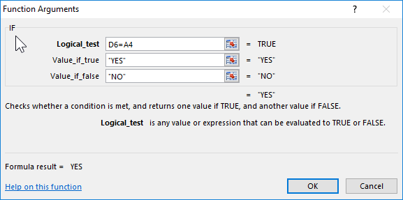
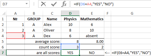
The specification of function arguments: = IF (). There are the number of all students in the cell A4, and in the cell D6 and E6 – the number of estimates. The IF () checks whether D6 and E6 are the same as A4. If functions are the same, we get the answer YES, and if not, the answer is NO.
In logical expression, there are 2 types of references are used for convenience: relative and absolute. This allows us to copy the formula without errors in the results of its calculation.
The notation. The «Formulas» tab provides access only to the most frequently used functions. You may get more by calling the «Functions Wizard» window by clicking on the «Insert function» button at the beginning of the formula line. Or we may press SHIFT + F3.
How to round numbers in Excel
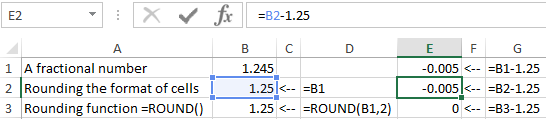
The = ROUND () is more accurate and useful than rounding by using a cell format. This is easily seen in practice.
- Make the original chart as shown in the picture:
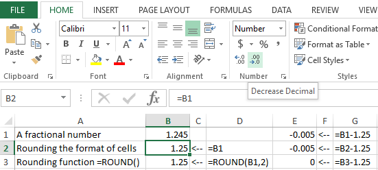
- The cell B2 you need format so, that only 2 decimal places are displayed. This can be done using the «Format cells» dialog box or the tool located on the «HOME» tab – «Decrease Decimal».
- In the column C you should add the subtraction formula of 1.25 from the values of column B: =B-1.25.
Now you know how to use the ROUND function in Excel.
The description of function arguments =ROUND():
- The first reason – is the cell reference to the value to be rounded.
- The second reason – is the number of symbols after point, that need to left after rounding.
Attention! The formatting cells only displays rounding, but does not change the value, and = ROUND () – rounds the value. Therefore, for calculations and computations, you need to use the function = ROUND (), inasmuch formatting of the cells will result in erroneous values in the meanings.
