Changing and aligning of fonts in cells
By default in Excel, the text is on the left side, and the numbers – on the right one. The change in these positions is sometimes justified, but often makes it difficult to distinguish a number from a text.
Treat to the text formatting with moderation. Do not forget, that a stylishly designed document should not contain more than 2 – 3 types of font. There should be no more than 2 – 3 colors, but more shades are allowed.
The changing of the default font in Excel
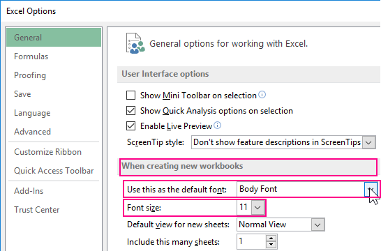
How in Excel to set the default font? For this you need to change 2 parameters in the settings:
- Go to the settings «FILE» – «Options» – «General».
- In the «When creating new workbooks» section, select the required «Font» from the drop-down list.
- Below specify its size and click OK.
The expanding of selected items
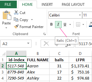
To show how to change the default font in Excel, we will format the text in the cells of the data table. The headings of the columns will be highlighted in bold and increase the size of the characters. The text data will be done in italic italics.
The solution of this task is no different from using the tools that Word has. The sequence of actions is as follows:
- Select the range with the column headings of the table.
- On the «HOME» tool tab, press the «B» (bold) button or the CTRL + B key combination.
- In the font size field, we click the mouse and enter our value – is 12, then click «Etner» (you can also specify the font size from the drop-down list of the field). On the same tab, click the «Align Center» button or the hotkey combination: CTRL + E.
- Now select the text data of table A2:B4 and click on the button «Italic» (CTRL + I).
This task can be solved in another way, using the «Format Cells» dialog box. It has more possibilities for formatting text in Excel.
- Again select the range A1 : D1.
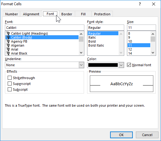
- Call the «Format Cells» dialog box using the corner button on the «HOME» tab in the «Align» tool section or press the CTRL + 1 (or CTRL + SHIFT + P) combination. We are interested in the «Font» tab:
- Here we can customize the text in the «Font» tab. In the «Inscription» field, select «Bold Italic». In the Size field, select or set the size to 14.
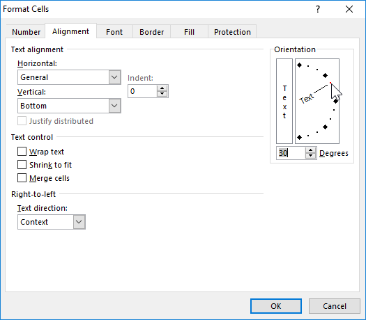
- Go to the «Alignment» tab.
- In the drop-down list «horizontally», set the value «centered». In the «vertical» list, specify «at the top».
Increase the height of line 1 approximately 2 times. Now you can see that the text of the table headings is centered and is adjacent to the upper edge of the cells.
The formatting the values of the cells helps us to make the data readable and presentable, that are easier to perceive and assimilate. For example, the number 12 can be formatted as 12 $ or 12% or 12 pcs.
In addition, the standard format «General» looks gray and not presentable, but it's also not too much to overdo it.
In the next lessons of this section, we'll take a closer look at the possibilities of formatting in Excel.
