Filling cells in Excel by the signs after decimal separator
When entering the values in Excel worksheet cells, all the data passes through the built-in software filter formatting. It allows you to simplify the work of user. Therefore, the entered data may differ from the displayed values after input.
To what problems can result the filter of formats of cells we will consider on the concrete examples, and also we will find to the best solutions for the exit from the prevailing situations.
If Excel considers incorrectly to the numbers after the decimal
Let`s consider the simple example where the contents of the cells are different from displaying its values. For example, mathematical errors can occur when fractional numbers are rounded down.
On the final example, we demonstrate to the following calculations.
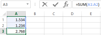
- You need to fill the original table as shown in the picture:
- In the cells B and C to set the Accounting format (CTRL + 1 «Format of Cells»-«Number»-«Accounting»).
- In the cell C1 you need to write down, what is displayed in the cell B1 (1.53-is the result after rounding up to two decimal places). In the same way you need to enter the number in C2 as it is displayed in B2 (the symbols of the currencies are not set, because its will be delivered automatically due to the accounting format).
- In the third line, you need to summarize the value of each column of the table.
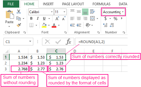
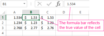
As you can see, the accuracy of calculating digits after a separator in Excel can be different. Formatting in reality does not round up the numeric values in the cells: they remain the same and the real ones are displayed in the formula bar.
When summing of a large number of such rounding off, errors can be very considerable, therefore in calculations and computations, you can`t round up with using formatting. You need to know how to round up the amount in Excel. The precise rounding can be done only by special functions such as:
- =ROUND();
- =ROUNDUP();
- =ROUNDDOWN();
- =INT() – (this function allows Excel to round to a larger integer).
For effectively using these functions in large quantities you can use arrays of functions, but this we is already covered in the following lessons.
The automatic insertion of a decimal point
The automatic filter of formats designed for simplify the work with the program, especially if you learn how to manage it. We have to put a separator when entering money to display cents very often. A decimal separator delimiter in Excel can be entered automatically when the accounting data is filled in monetary terms. For this:
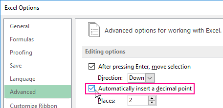
- Open the window «File»-«Options».
- In the window «Excel Options you need to go to «Advanced»-«Editing options» and tick the box «Automatic insertion with a decimal point». The number of characters after the delimiter should remain «2». Now you need to check the result.
- In the cell A1, enter 1234 and press «Enter»: as a result we see 12, 34 as in the picture:
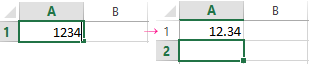
Now you can easy enter the amount with cents, without separating them with a separator. After each input, the separator will be automatically inserted before the last two numbers.
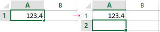
It should be noted that if in the amount of 00 cents, the signs after the separator in Excel must be entered necessarily. Otherwise, it can turn out like 0.01 or 0.2.
If you enter a separator with the automatic separator insertion mode, it will remain in the place where you entered it.
That is, the number of decimal places can be changed or moved to the separator itself.
After filling the amounts with cents do not forget to disable this function.
