Automatic recalculation of formulas in Excel and manually

Excel by default recalculates all formulas in all sheets of all open books after each introduction of data. The most swell possibility of Excel – is the automatic recounting by formulas. If the sheet contains hundreds or thousands of formulas, the automatic recalculation starts to noticeably slow down the process of working with the program. This ability of spreadsheets increased people's productivity in dozens of times.

After all, with manual calculation we need to enter each time not only numbers but mathematical operations, do not get confused, constantly placing intermediate results in memory and so on. In our case, we create formulas and then simply change the numbers - everything will automatically be counted again. Well, if the changes are small, it is even better - even to introduce less of data.

Let`s contemplate, how you can customize Excel to improve its performance and unhindered working.



Automatic and manual conversion

For a book that contains hundreds of compound formulas, you can turn against to the recalculation on requirement of a user. For this:

1. You need to enter the formula on a blank sheet (so that you can check how this example works).
2. You need to select the tool: «Formulas» – «Calculation Options» – «Manual».
3. Make sure that now after entering the data into the cell (for example, the number 7 instead of 1 in the cell A2 as in the draught), the formula does not automatically recalculate the result – while the user does not press the F9 key (or SFIFT + F9).

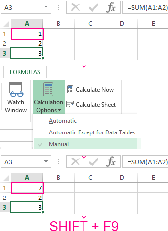
Pay attention! The shortcut F9 performs recalculation in all book formulas on all sheets. There is Combination of hot keys SHIFT + F9 performs recalculation only on the current sheet.

If the sheet does not contain a lot of formulas, that`s why the recalculation can inhibit to Excel. That`s why it makes no sense to use the above described example, but for the future it still worth knowing for you about this possibility: because after all, over time you will have to deal with complex tables with a lot of formulas.

Furthermore, this function can be turned on accidentally and you need to know where to turn it off for the standard operating mode.



How to display to a formula in the Excel cell

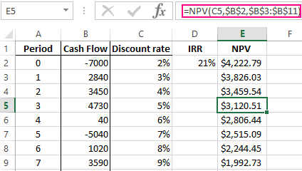
In the Excel cells, we can see the result of the calculations only. The formulas themselves can be seen in the formula line (separately). But sometimes we need to simultaneously view all functions in cells (for example, to compare them, and so forth).

To visually display the example of this lesson, we need this sheet containing the formulas:

We change the Excel settings accordingly so that the cells display the formulas, but not the result of their calculation.

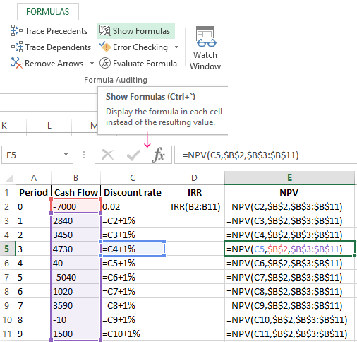
To achieve this result, you need to select the tool: «Formulas» – «Show Formulas»» (in the section «Formulas Auditing»). To exit this display mode, you should to select this implement again.

You can also use the shortcut keys combination CTRL + `(above the Tab key). This combination works in switch mode, that is, you need to press this key repeatedly and returns to the normal display mode of calculation results in cells.

The notation. All the above described actions apply only to the mode of displaying cells of one sheet. That is, on other sheets, if necessary, you need to perform these actions again.