Sampling of values from the Excel table by condition
If you have to work with large tables you definitely will find in ones duplicate sums, that scattered along the whole column. At the same time, you may need to select data from the table with the first smallest numerical value that has its own duplicates. You need automatic sampling of data by condition. In Excel for this purpose, you can successfully use the formula in the array.
How to make the sample in Excel by condition
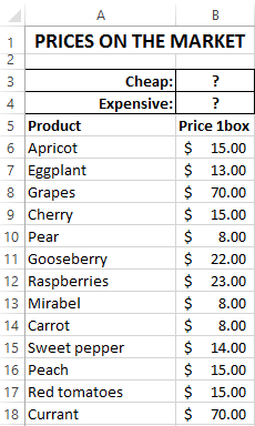
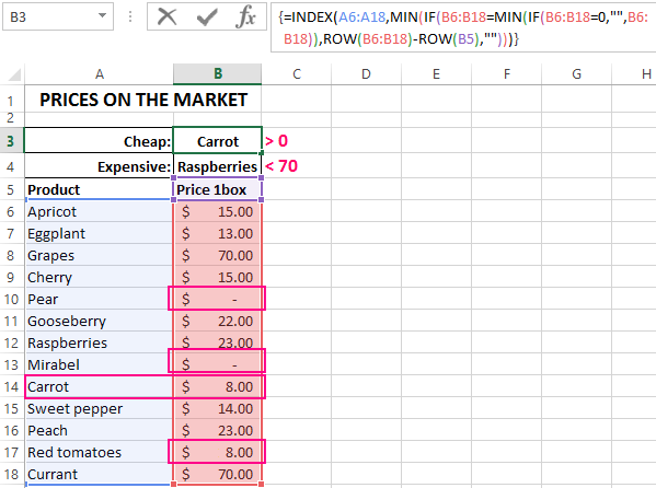
To determine the corresponding value, to the first smallest number needs to be fetched from the table by condition. Let's say we want to know the first cheapest product on the market from this price list:
The automatic sampling implements will be the formula with the following structure:
INDEX(data_range_for_sampling, MIN(IF(range=MIN(range), ROW(range)-ROW(column_header),””)))
In the place «range_data_for_sampling» you need to specify the A6:A18 range of values for the selection from the table (for example, text), from which the INDEX function will sample one result value. The argument «range» means a region of cells with numerical values, from which the first smallest number should be selected. In the «column_header» argument for the second ROW function, you must specify the reference to the cell with the column header that contains the range of numeric values.
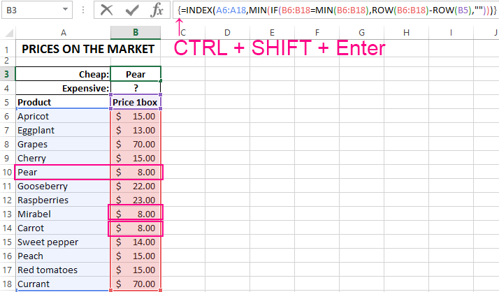
Naturally, this formula should be executed in an array. Therefore, to confirm its input, so you should press not just the Enter key, but the whole combination of the keys CTRL + SHIFT + Enter ({}). If everything is done correctly, the braces will appear in the formula line.
Note the figure below, where the formula was entered in the cell B3 in the array ({}):
The sample of the corresponding value with the first smallest number:
With this formula, we were able to choose the minimum value with respect to numbers. Next, we will analyze the principle of the formula and step-by-step to analyze the entire order of all calculations.
How does the sampling by condition
The key role here is played by the INDEX function. Its nominal task is to select from the source table (it indicated in the first argument – A6:A18) values, that corresponding to the certain numbers. The INDEX works with the criteria specified in the second (the row number within the table) and in the third (the column number in the table) arguments. Since our source table A6:A18 has only 1 column, we do not specify the third argument in the INDEX function.
To calculate the row number of the table opposite the smallest number in the adjacent range is the B6:B18 and use it as the value for the second argument, when several computational functions are used.
The IF function allows you to sample the value from the list by condition. In its first argument, it specifies where each cell in the B6:B18 range is checked for the lowest numerical value: IF6:B18 = MIN6:B18. In this way, the array is created in the program memory from the logical values TRUE and FALSE. In our case, 3 elements of the array will contain the value TRUE, since the minimum value of 8 contains 2 more duplicates in the column B6:B18.
The next step is to determine which line of the range each minimum value is in. We need this because of the determination of the first lowest value. This task is implemented using the ROW function, it fills the elements of the array in the program memory with line. But first, from all these numbers, the number on the first row of the table is subtracted – B5, that is, the number 5. This is done because the INDEX function works with numbers inside of the table, and not with the numbers of the Excel worksheet. At the same time, the ROW function can only return line number of the sheet. To prevent the offset from occurring, you need to match the order of the line number and the number of the table by subtracting the difference. For example, if the table is on the 5-th row of the sheet, each row of the table will be 5 less than the corresponding line of the sheet.
After all the minimum values have been selected and all the rows of the table are matched, the MIN function will select the smallest line number. The same line will contain the first smallest number that occurs in column B6:B18. Based on this line number, the INDEX function will select the corresponding value from the table A6:A18. As a result, the formula returns this value to the cell B3 as the result of the calculation.
How to select the value with the largest number in Excel
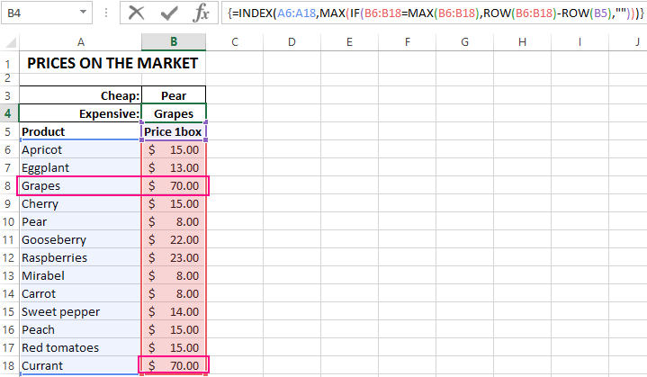
Understanding the principle of the formula, you can now easily modify it and adjust it to other conditions. For example, you can change the formula to select the first maximum value in Excel:
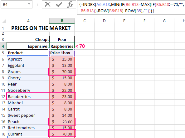
If you need to change the conditions of the formula so that you can select the first maximum in Excel, but less than 70:
As in Excel you can select the first minimum value except of zero:
As it easy to see, these formulas differ only in the functions of MIN and MAX and ones arguments.
Download sampling of values from table in Excel.
Now nothing restricts of you. Once you understand to the principles of the action of formulas in an array, you can easily modify ones under the variety of conditions and quickly solve a lot of computational problems.
