VLOOKUP function with multiple criteria conditions in Excel
The VLOOKUP (Vertical Look Up) function searches in the data table and based on search query criteria, returns the corresponding value from the specific column. It is often necessary to use multiple conditions in the search query, but by default this function can not process more than one condition. Therefore, you should use a very simple formula that will extend the capabilities of the VLOOKUP function across several columns simultaneously.
The function of the VLOOKUP function by several criteria
For clarity, we will discuss the VLOOKUP formula with the example of several conditions. For example, we will use the schematic report on the revenue of sales representatives for the quarter:
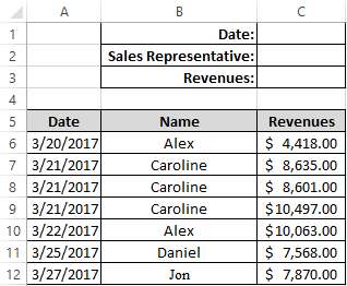
In this report, you need to find to the revenue figure for a certain sales representative in the certain date. Given the search terms, our request must contain 2 conditions:
- – The date of delivery of proceeds to the cashier.
- – Name of the sales representative.
To solve this problem, we will use the VLOOKUP function for multiple conditions and compose the following formula:
- In the cell C1 to enter the first value for the first search query criterion. For example, the date: 03.22.2017.
- In the cell C2 to enter the name of the sales representative (for example, Alex). This value will be used as the second argument of the search query.
- In the cell C3 we will get the result of the search, for this we need to enter the formula:
- After entering the formula, you need to press the combination of the hot keys CTRL + SHIFT + Enter ({}) for confirmation, because this formula must be executed in the array.
The result of the table search is based on two conditions:
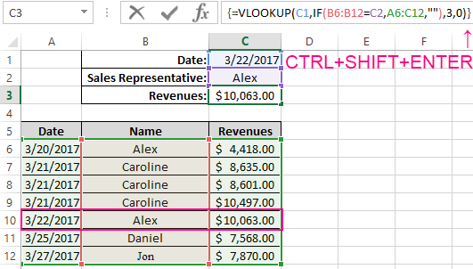
The amount of revenue of the specific sales representative for the specific date was found.
The analysis of the principle of the formula`s action for the VLOOKUP function with multiple conditions:
The first argument of the function = VLOOKUP(). It is the first condition for finding the value according to the table of the sales revenue report. The second argument contains to the virtual table, that was created as the result of the massive calculation by the logical function = IF(). Each name in the range of the cells B6:B12 is compared with the value in the cell C2. Thus, the conditional data array with TRUE and FALSE value elements is created in memory.
Then thanks to this formula, in the memory of the program each true element is replaced by the 3-element data set:
- Element - the Date.
- Element – the Name.
- Element – the Revenue.
And each false element in memory is replaced by the 3-element set of empty text values (""). As a result, a new table is created in the program memory, with which the VLOOKUP function will already work. It ignores to all empty sets of data elements. And non-empty elements are mapped to the value of the cell C1, that used as the first criterion of the search query (Date). In one word, the table in memory is checked by the VLOOKUP function with one search condition. With a positive result of the mapping, this function returns the value of the element from the third column (revenue) of the conditional table. This is because the third argument specifies the number of the column 3, from what the values are taken. It is worth noting, that to view the arguments of the function the entire table is specified (in the second argument), but the search itself always follows the first column in the specified table.
Download example VLOOKUP function with multiple conditions in Excel.
And from which column to take the return value, is indicated already in the third argument.
The number 0 in the last argument of the function indicates, that the match must be absolutely exact.
