How to fix a row and column in Excel when scrolling
The Microsoft Excel program is designed not only to enter data into the table conveniently and edit it as you need it, but also to view large blocks of information. Most people using PCs work with it constantly.
The columns and rows names can be significantly removed from the cells with which the user is working at this time. Scrolling the page to see the name of the document is not comfortable for any user. Therefore, the Tabular Processor has possibilities to fix certain areas.
Locking a row in Excel while scrolling
Usually an Excel table has one cap. Meanwhile, this document can have up to thousands of rows. Working with multipage table blocks is inconvenient when column names are not visible. Scrolling the page to its beginning to return to the correct cell is absolutely irrational. To make the cap visible when scrolling, fix the top row of the Excel table, following these actions:
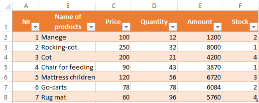
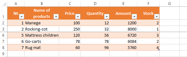
- Create the needed table and fill it with the data.
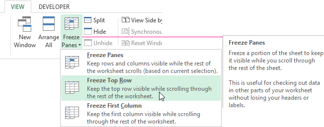
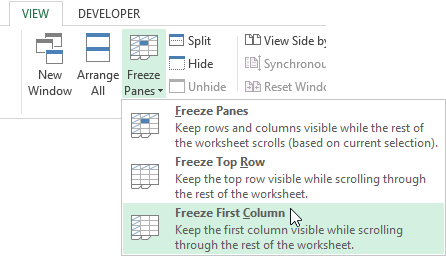
- Make any of the cells active. Go to the “VIEW” tab using the tool “Freeze Panes”.
- In the menu select the “Freeze Top Row” functions.
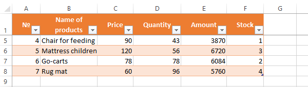
You will get a delimiting line under the top line. Now when you scroll vertically the table cap will be always visible.
Locking several rows in Excel while scrolling
Let us suppose, a user needs to fix not only the cap. For instance, another row or even a couple of rows must be fixed when scrolling the document. Doing it is possible and easy, when you follow these steps:
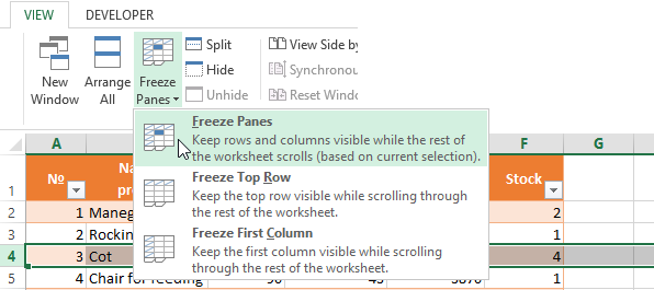
- Select any cell under the line, which we will fix. This action will help Excel to “understand”, which area should be fixed;
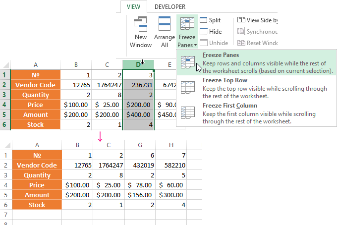
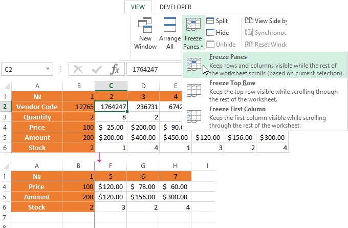
- Now select the “Freeze Panes” tool.
When you perform horizontal and vertical scrolling, the cap and the top row of the table remain fixed. Thus, you can fix two, three, four and more rows.
Note: This method works for 2007 and 2010 Excel versions. In earlier versions the “Lock areas” tool is located in the “Window” menu on the main page. There you must always (!) activate the cell under the freeze row.
Freezing columns in Excel
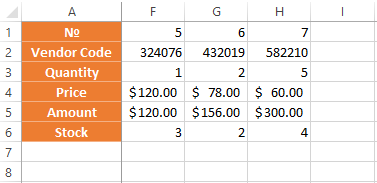
For instance, the information in the table has a horizontal direction. It is not concentrated in columns, but located in rows. For his comfort, the user must freeze the first column, containing the lines’ names in horizontal scrolling.
- Select any cell of the chosen table so that Excel understands with what data it will work. Pin the first column in the menu you will see..
- Now, when the document is scrolled to the right horizontally, the needed column will be fixed.
To freeze several columns, select the cell at the page bottom (to the right from the fixed column). Pick the “Freeze Panes” button.
How to freeze the row and column in Excel
You have a task – to freeze the selected area, which contains two columns and two rows.
Make a cell at the intersection of the fixed rows and columns active. However, the cell must be not placed in the fixed area. It should have the position right under the required lines (to the right of the required columns). Pick the first option in Excel Locking Areas. The photo shows that when scrolling, the selected areas remain at the same place.
Removing a fixed area in Excel
After fixing a row or a column of the table the button deleting all pivot tables becomes available.
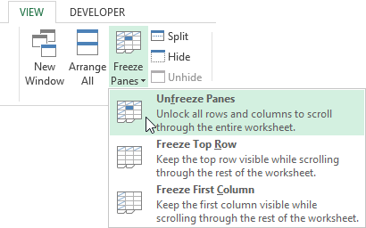
After clicking – «Unfreeze Panes», all the locked areas of the worksheet become unlocked.

Download beautiful templates and speed up report creation in Excel.
Download Templates