How to remove Gridlines in Excel for specific cells
The Excel workspace is a table that consists of columns, rows, and cells. Visually everything is displayed as an entire grid. In some tasks when creating document forms or for creating special templates and interfaces, the grid interferes and needs to be removed.
Hiding the Sheet Gridlines
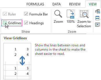
In all new versions of Excel, starting from 2007, the gridlines can be disabled from the toolbar: «VIEW». In the «Show» section you need to uncheck the «Gridlines» option.
There are two more ways to remove the grid Excel table:
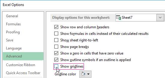
- Program settings. «FILE»-«Options»-«Advanced»-«Display options for this worksheet:» remove the checkmark from the option «Show gridlines».
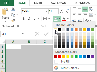
- Press the combination of hot keys CTRL + A to select all the cells in the sheet. On the tab of the «HOME» tool bars, select the «Theme Colors» tool and specify the white color. To return the gridlines, you must select everything again and change it from white to «No Fill». This method will remove the grid in any version of Excel.
The second way is interesting because it can partially (selectively) remove the gridlines.
How to delete gridlines in Excel
You need to select not a whole sheet, but the ranges in those areas of the document where you want to remove the Excel grid. The truth for beauty will need to change the extreme boundaries of cells. The default colour code for the cells of the grey background gridlines is:
- RGB (218, 220, 221);
- HTML #DADCDD.
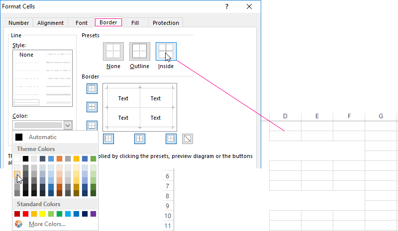
Note. The cell borders change in the «Format Cells» dialog box on the «Borders» "Borders" tab, and press CTRL + SHIFT + F (or CTRL + 1) to call it.

Download beautiful templates and speed up report creation in Excel.
Download Templates