How to quickly move the cursor to the Excel sheet cells

Moving on the sheet cells is carried out with the help of the cursor (controlled black rectangle). Most often, you need to move to the next cell when you fill in the Excel worksheets. But sometimes you need to move to any remote cells.

For example, you need to move to the end / start of the price list, etc. Each cell under the cursor is active. Viewing the contents of Excel worksheets can be divided into 2 types: first view by moving the cursor and the second view with the help of additional tools intended for viewing without moving the cursor. For example, the scroll bars of the sheet.

How to quickly move through cells in Excel with arrows keys is described in more detail below.



Moving the cursor to the next cell in the bottom

Move the cursor to the bottom (next) cell. When the program is loaded by default, the cursor is located on the cell with the address A1. You need to go to cell A2. There are 5 options for this solution:

1. Just press the "Enter" key.
2. Moving between the cells by using arrows keys. (All the arrows on the keyboard affect the movement of the cursor respectively with its direction).
3. Point your mouse at the cell with address A2 and click the left mouse button.
4. Use the "Go To" tool (CTRL+G or F5).
5. Using the "Name" field (located to the left of the formula line).

Over time, in the process of working with Excel, you will notice that each option has its own advantages in certain situations. Sometimes it is better to click, and sometimes it's better to move the cursor with the "Enter" key. Also, an additional example can serve this task and show how you can find solutions in several ways in Excel.

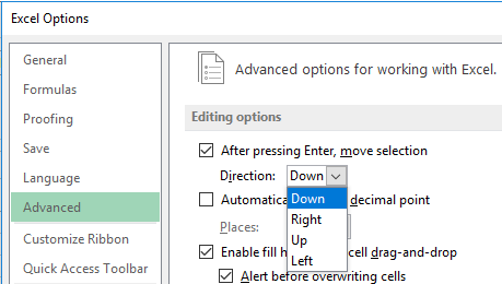
By default, the parameter for moving the cursor in Excel after pressing the "Enter" key is directed to the bottom, to the bottom cell (and if you press SHIFT+ENTER, the cursor will go to the top cell). If necessary, this can be changed in the program settings. Open the "Excel Options" window through the "FILE" - "Options" menu. In the opened window select the "Advanced" option. We are interested here with this option: "After pressing Enter, move selection Direction:". Below in the option specify the direction you want as shown in the picture:

Remember that the changes in this setting will make your work in Excel more comfortable. In certain situations of filling / changing data, you will often have to use this feature. It is very convenient when the cursor itself moves in the desired direction after entering data into the cell. And tables in sheets for data filling can be both vertical and horizontal.



Fast jump to selected remote cells

We moved along neighboring cells (C A1 to A2) in the above-described example. Try in the same way to move the cursor (black rectangle) to cell D3.

As you can see, in the given task the shortest way is to make 1 click with the mouse. After all, for the keyboard, it is 3 keystrokes.

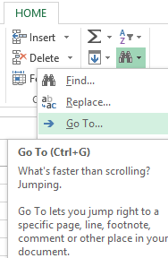
To solve this task, you can also use the "Go To" tool. To use it, you need to open the drop-down list of the "Find" tool on the "Home" tab and select the "Go To" option. Or you can press the combination of the hotkeys CTRL+G or F5.

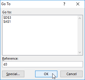
In the opened window enter D3 (you can enter it with small letters d3, and the program itself replaces small letters in large letters and in formulas it works in the same way), then click OK.

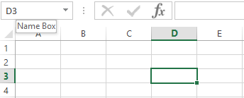
To quickly move the cursor to any address of a worksheet cell, it is also convenient to use the "NameBox" field which is in the upper left corner under the tool bar at the same level as the formula line. Enter in this field D3 (or d3) and press "Enter". The cursor will instantly move to the specified address.

If the remote cell to which the cursor should be moved to make it active is situated in the same screen (view without scrolling), then it is better to use the mouse. If the cell needs to be searched but its address is known in advance, it is better to use the "NameBox" field or the "Go To" tool.

Most functions in Excel can be implemented in several ways. But in the further lessons, we will use only the shortest.

Move the cursor to the end of the worksheet

On a practical example, we quickly check the number of rows in a sheet.

Task 1. Open a new worksheet and place the cursor in any column. Press the END key on the keyboard, and then the "down arrow" (or use the combination of CTRL+"down arrow"). And you will see that the cursor has moved to the last line of the worksheet. If you press CTRL+HOME, the cursor moves to the first A1 cell.

Now check the address of the last column and number of columns.

To find out which column is the last in the worksheet, you must change the display style of the cells link addresses. To do this, go to "FILE" - "Options" - "Formulas" and tick the "R1C1 reference style" and then click OK.

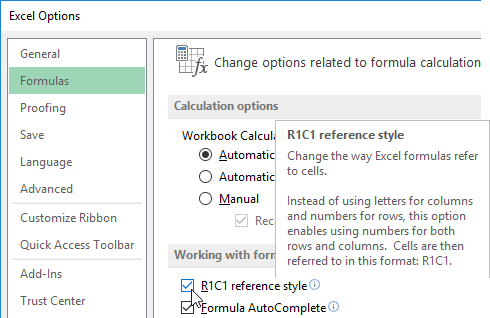
After that, the names of the columns will be replaced by numbers instead of letters. The sequence number of the last column of the sheet is 16384. After that, in the same order, uncheck the box to return the standard style of the columns with Latin letters.

The Excel ancestor was a program in the of a calculator-sheet style to help with work in the accounting department.

Therefore, the sheets resemble one large table. Now we have learned how to effectively navigate through the cells of this table, and then we will learn, how to effectively fill them with data.