Examples of using the FIND function in Excel Formulas

The LEFT, RIGHT, and MID functions are excellent for splitting strings into words or text fragments, but only if you already know the positions of the characters from which the split will occur. What if you don't know in advance where the character is in the text string from which you need to extract a text fragment?



Example of FIND, LEN, and RIGHT functions in Excel

Suppose you have a price list with product codes, and you want to extract the characters after the hyphen from each code, but the hyphen is in a different position in each code. How do you achieve this?

• PTR-422
• CORPO-6755
• SVCCALL-56532

The LEFT function is not suitable since we need the last part of each code. The RIGHT function also cannot handle this task because it requires specifying the exact number of characters to return, and the codes have different lengths. If a fixed numerical value is specified in the argument, it may work for some codes but not for most, resulting in too many or too few characters returned by the RIGHT function.

In practice, it is often necessary to automatically find a specific character so that the function itself determines the starting position for extracting a text fragment from the original string.

To implement this task, you should use a formula with a combination of the RIGHT, LEN, and FIND functions:

=RIGHT(A2,LEN(A2)-FIND("-",A2))

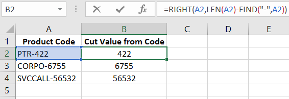
Thanks to the FIND function, you can automatically determine the position in the text string for the specified character in its arguments. After that, you can use the position number in subsequent operations, for example, when automatically generating values for the second argument of the RIGHT function. The generation is done by determining the required number by subtracting from the length of the string returned by the LEN function the position number of the character "-".

Example of using FIND and MID in an Excel formula

In the next example shown in the image, the FIND function is used in a formula along with the MID function to extract the middle numbers between hyphens from the product code in the price list.

=MID(A2,FIND("-",A2)+1,2)

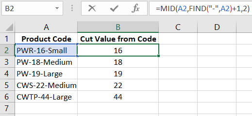
As seen in the image, the formula first finds the position number for the character using the FIND function. After finding the position number, it is used in the arguments of the MID function.

The FIND function requires filling in a minimum of 2 out of 3 arguments:

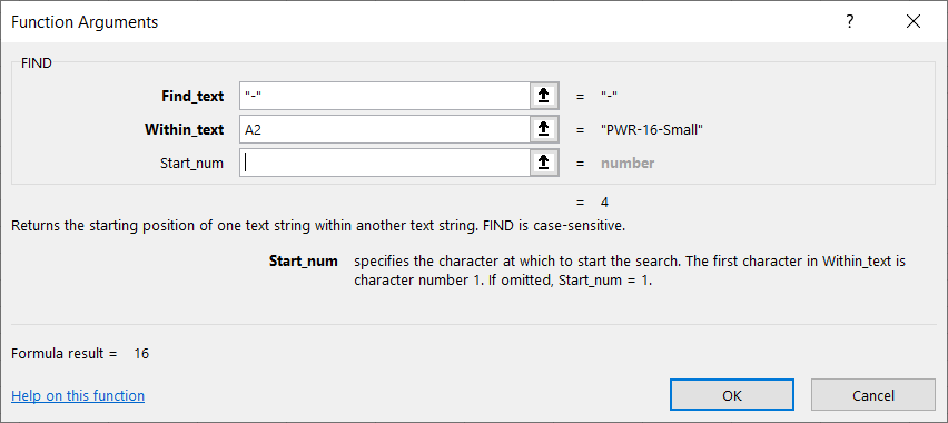
1. Find_text – here you need to specify the text to find and get its ordinal number (position) in the original text string.
2. Within_text – here you specify the reference to the cell with the original string that contains the searched character or text.
3. Start_num – this is an optional argument. Here you can specify the position number of the character in the string from which to start the search. If the string contains more than one found character, using this optional argument allows specifying the number of the character from which the rest of the string will be viewed. If it is not specified in this argument, it defaults to = 1, meaning from the first character, and thus the entire string.

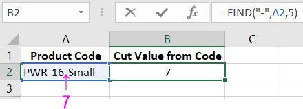
For example, in the example, the function finds the first hyphen in the string "PWR-16-Small". As a result of its calculation, it returns the number 4 by default since the first hyphen in the original string is at the fourth position.

Dynamic formulas using the FIND function

But if we use the third optional argument and specify the number 5 in it, i.e., to start viewing not from the beginning but after the first hyphen, the fourth character. Then the function will return the ordinal position of the second "-", i.e., the number - 7.

The FIND text function is most often used as a helper by specifying it as an argument for other text functions. For example, if we use it as the second argument for the MID function, we get the ability to cut a text fragment of different lengths, automatically determining the required position in the string as a marker for separating its part.

If we use the formula mentioned in the example, we cut 2 numeric characters located after the first hyphen from each product code. Note the addition in the formula +1, which shifts the focus of the function by one character to determine its position on characters after the hyphen (bypassing it).

As mentioned earlier, by default, the FIND function returns the position of the first found character in the original viewed text string. When we need to find the second occurrence of the same character and know its position in the string, we can use the optional third argument of the function. In this argument, you can specify the position of the character in the original string from which to start the search.

For example, the following formula returns the position of the second hyphen, as the third argument specifies the position number of the first hyphen. This means that the search will be conducted not throughout the string but only in its part starting from the first hyphen.

=FIND("-",A2,FIND("-",A2)+1)

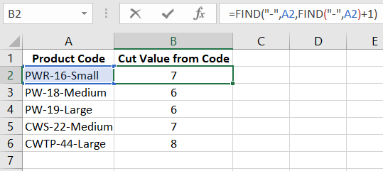
Thus, we have created a dynamic formula that automatically determines where (at which position) the first and second hyphens are in the string. And then they can be used as arguments in other functions.

An example from the practical experience of an office employee. It is necessary to get part of the product codes that starts from the second hyphen. To do this, we create a dynamic formula:

=RIGHT(A2,LEN(A2)-FIND("-",A2,FIND("-",A2)+1))

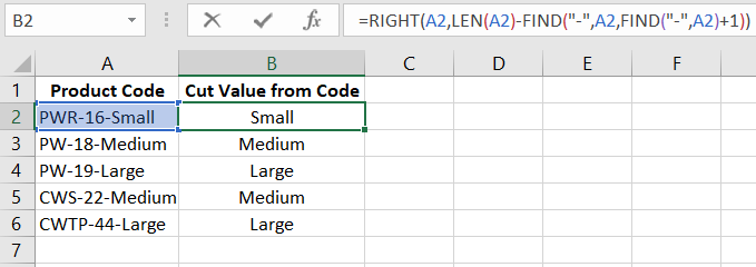
Here, we used automatic search for the first hyphen. The position number served as the third optional argument of the FIND function for automatically searching for every second hyphen in each product code. Then, using the LEN function, we determine the length of the original string and subtract from it the number of positions of the second character. In other words, subtracting the length of the code from the number of characters to the second hyphen (including it, as indicated by the addition +1). Thus, we dynamically determine the second argument for the RIGHT function to cut text fragments of varying lengths from the strings. Moreover, all the strings have different lengths, and the second hyphen is also in different places. But the smart formula handled it completely automatically.

Example of Inexact Search with the FIND Function in an Excel Table Column

In the database of a retail-focused enterprise, all products are labeled with special codes! The structure of each code looks like this:

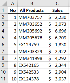
1. The first two characters represent the main category: MM - Mass Market or EX - Exclusive Products.
2. Three characters starting from the third symbol of the code correspond to the product subcategory (for example, 703 - wood tools, 205 - metal tools, 124 - wind generators).
3. All other digits are the manufacturer's code.

It is required to create a selection of sales indicators for products based on indirect criteria and with inexact search. For example, to avoid separately entering the ID code for each product like MM703757, but only entering common values in the code like 703 or MM. The formula algorithm should be able to understand all similar properties in the codes of similar products related to a particular category or subcategory.

To solve this challenging task, a formula should be created, with the useful FIND function at its core:

=IFERROR(INDEX($C$2:$C$11,INDEX(IF(IFERROR(FIND($F$1,$B$2:$B$11),0),ROW(INDIRECT("1:"&ROW())),""),A2)),0)

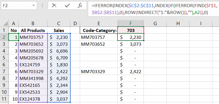
Now, simply enter a part of the code into cell F1, and the formula algorithm will find all codes based on indirect criteria:

Download

As seen from the examples described above, in the office environment, it is very common to use such a simple FIND function to solve complex and popular tasks.