How to find smallest positive or largest negative number in Excel range
Often, in a range of cells, both positive and negative numbers are found together. It's necessary to determine extreme values but with specific conditions. You should find the smallest value for positive numbers and separately for negative ones. To solve this problem, it's not enough to simply use functions like =MIN(), =MAX(), =SMALL(), or =LARGE(). Otherwise, when these functions are applied to a range with mixed positive and negative numbers, only the smallest negative value will be returned. Therefore, you should use a special formula with functions.
Smallest Positive Number
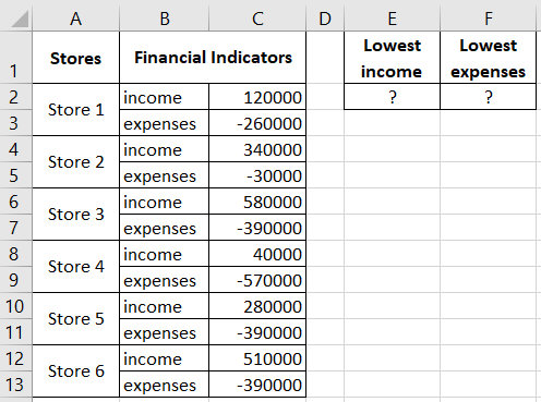
Let's say you have income and expenses statistics for a network of stores for a month. You need to find out which of the stores are the least costly in terms of expenses and the least profitable in terms of income. To present the solution, let's use an example table with income and expenses for the stores, as shown in the image below:
First, you should find the smallest income. To do this, the formula should first consider a group consisting of only positive numbers. Then, find the smallest positive value. To achieve this:
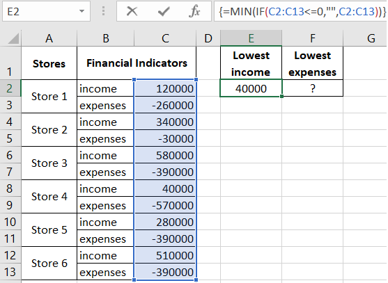
- In cell E2, enter the formula:
- After entering the formula, to confirm it, press the keyboard shortcut: CTRL+SHIFT+Enter, as it needs to be executed as an array formula. If done correctly, you'll see curly braces in the formula bar.
=MIN(IF(C2:C13<=0,"",C2:C13))
Explanation of how the formula works to find the smallest positive number:
The logical function =IF(), which is executed in an array formula, checks each cell in the range C2:C13 to see if it contains a number less than or equal to zero (<=0). Thus, a conditional table is created in memory with logical values:
- FALSE – for positive numbers (in this case, including zero);
- TRUE – for negative numbers.
Then, in the conditional table, the IF function replaces all TRUE values with blanks (""). Instead of the FALSE values, it puts the same positive numbers that were in the range C2:C13. The =MIN() function, which finishes the formula, returns the smallest positive number from the filtered table (already filtered from negative values and zeros).
Largest Negative Number in the Cell Range
To find the smallest expenses among negative values, specify the largest one. To do this, follow these steps:
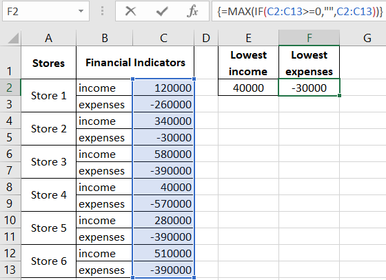
- In cell F2, enter the following formula:
- Just like the previous formula, after entering it, press the keyboard shortcut: CTRL+SHIFT+Enter, as it should be executed as an array formula. If done correctly, you'll see curly braces in the formula bar.
=MAX(IF(C2:C13>=0,"",C2:C13))
This is how you can use these formulas to select values from a database based on criteria:
 Download
As a result, we quickly and easily identified the least profitable store in terms of income, which is #4. And the least costly store in terms of expenses is store #2.
