Formula Formats Text and Number in Single Excel Cell

Often in Excel reports, it's necessary to combine text with numbers. The challenge is that, during the merging of text with a number, the numeric data cell cannot retain its numeric data format. The number in the cell is formatted as text.



Format a Number as Text in Excel with Currency Cell Format

Consider, for example, a report depicted below. Suppose you need to place a list of stores and their sales results in a single cell:

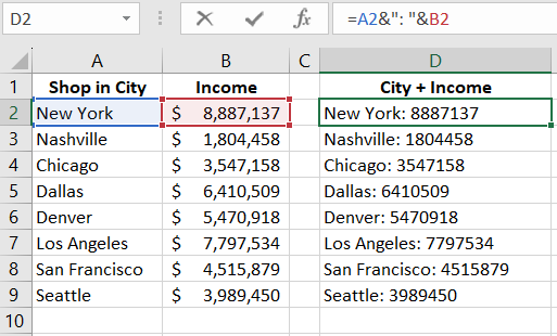
Note that each number, after being combined with text (in column D), does not retain its currency format defined in the original cell (column B).

To solve this problem, you need to reference the cells with numeric currency amounts into the TEXT function. This function allows formatting numeric values directly in the text string. The formula is shown below:

=A2&": "&TEXT(B2,"$ # ##0")

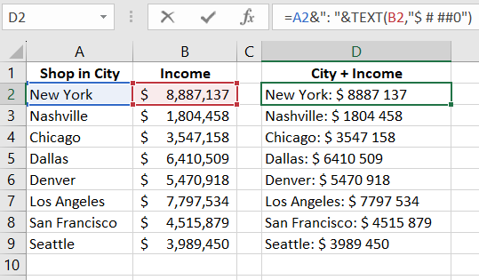
The formula solves this problem when dealing with a single currency type. When there are multiple currencies, a macro function must be used in the formula – this will be discussed later. For now, let's break down this formula.

The TEXT function requires two mandatory arguments:

1. Value – a reference to the original number (in this case).
2. Format – the text-based Excel cell format code (can be custom).

The number can be formatted in any way; the important thing is to follow the formatting rules recognized by Excel.

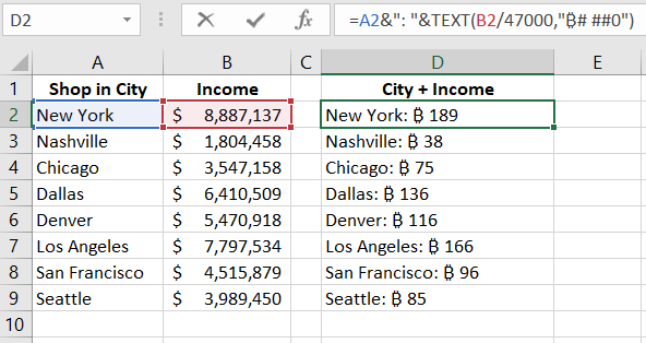
For example, the modified formula below returns the amount in the currency format recalculated at the rate of 47,000 dollars per 1 bitcoin:

=A2&": "&TEXT(B2/47000,"₿# ##0")

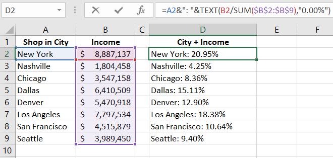
The adjusted formula below returns the percentage share of total revenue:

=A2&": "&TEXT(B2/SUM($B$2:$B$9),"0.00%")

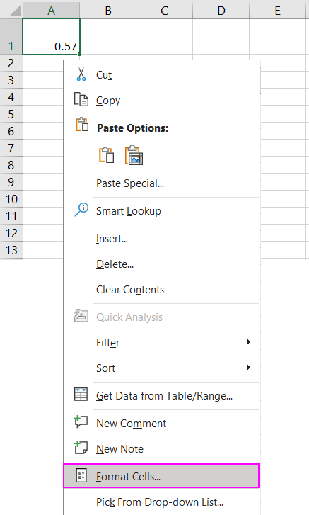
A simple way to check the syntax of the format code that Excel recognizes is to use the "Format Cells" window. To do this:

1. Right-click on any cell with a number and select "Format Cells" from the context menu. Alternatively, press the keyboard shortcut CTRL+1.

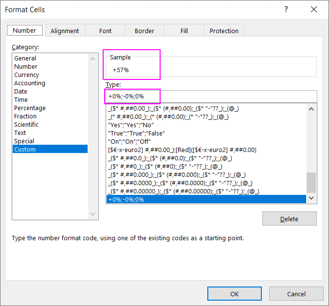
2. Go to the "Number" tab.

3. In the "Category" section under "Number Formats," choose the "(all)" category.
4. Enter your custom format code in the "Type:" field and observe how it is recognized by Excel and displayed in the cell in the "Sample" section.

DOLLAR Function for Formatting Numbers as Text in a Single Cell

A simpler alternative solution for this task can be the DOLLAR function, which converts any number to text and displays it in the currency format:

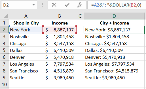
This solution is quite limited in functionality and is suitable only for cases where the combined number with text represents a monetary sum in dollars (or the default currency specified in the regional settings of the Windows control panel).

The DOLLAR function requires only two arguments to fill in:

1. Number – a reference to the numeric value (a required argument to fill in).
2. [Decimal_places] – The number of digits to the right of the decimal point.

Custom Macro Function to Get Cell Format in Excel

If the original column contains values in cells with different currency formats, we need to recognize all formats in each cell. By default, Excel lacks a standard function that can recognize and return cell formats. Therefore, let's write our custom macro function and add it to our formula. The macro function will be named GETFORMAT (or you can name it as you like). The original VBA code of the macro function looks like this:

Public Function GETFORMAT(val As Range) As String
Dim money As String
money = WorksheetFunction.Text(val, val.NumberFormat)
GETFORMAT = Replace(money, Application.ThousandsSeparator, " ")
End Function


Copy it into the module ("Insert"-"Module") of the VBA editor (ALT+F11). If necessary, read:

Example of how to create a macro in Excel.

Now modify our formula and get the most efficient result:

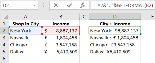
Thanks to the GETFORMAT function written in VBA macro, we simply take the value and format from the original cell and substitute it as a text string. Thus, our formula with the custom macro function GETFORMAT automatically determines the currency for each sum in the original cell values.

Example Presentation of Text Formatting Using Formulas

In practice, it is very common to dynamically format text using Excel functions, especially in the process of developing data visualizations. As an example, let's simulate a situation. We need to develop a simple game in Excel using standard charts and formulas. Without using macros! At the same time, the player's performance label should be displayed in percentage data format with positive (+) and negative (-) values. Depending on the player's position above or below sea level:

Download

As seen, the format of the label text on the chart dynamically changes depending on the game process. With the maximum jump, the value returns in the format +100%, and with the minimum jump, -100%. When the player is at sea level, the value is returned as 0% without signs (+) or (-). The entire game concept is implemented in Excel using standard charts, formulas, and functions without using macros.