Excel formulas for dynamic asset summation in reports

For many reports, the current sum is often used, which is defined as the indicator of changes in a certain value over a period of time.



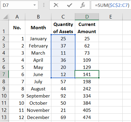
Formula for summing current assets

Below is an example of the current sum of the number of assets acquired over a period of time for a year, from January to December. The formula used in cell B2 is copied to all cells for the remaining months:

=SUM($C$2:C2)

Done!

In this formula, the SUM function is used to sum values starting from cell B2 up to the current month. The elegance of using the SUM function in this example lies in locking the absolute address of the reference only to the first cell of the range specified as an argument to the function. Thanks to this trick, the SUM function sums the range of cells from the first $B$2 to the cell of the current month. All ingenious is simple.

How and where to apply the formula for dynamic summation in Excel?

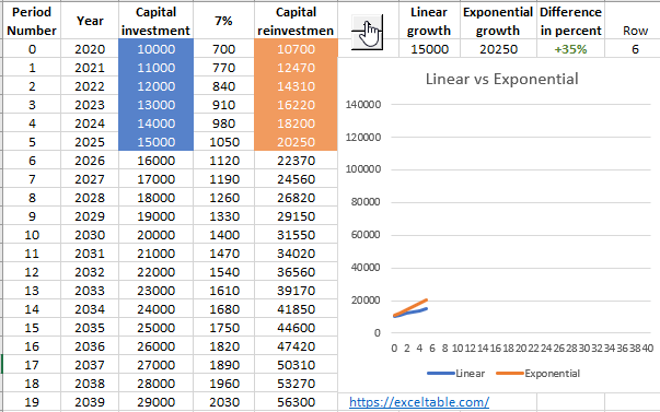
Let's consider a simple example. It is necessary to compare the difference in the return levels of two investment portfolios with linear and exponential methods of capital accumulation over 40 years.

Linear method of capital accumulation

Suppose $10,000 is invested in an investment object, for example, the ETF S&P500, with an average annual return of 7%. According to the investment portfolio plan, additional funds will be accumulated annually, on average, by $1000. This is a linear method of capital accumulation.

Exponential method of capital reinvestment

According to the plan for the second portfolio, the initial contribution is also $10,000, the investment object is the same ETF S&P500 with an average annual return of 7%. The annual replenishment has also not changed and is the same + $1000 per year. But the main difference is the annual reinvestment of all the profit received from the investment object ETF S&P500.

Technical Task for the investor: it is necessary to compile a planned history of future profits and capital accumulation in an Excel table according to the investment plan. It is also necessary to create a simple but readable data visualization from a chart with two curves:

1. Linear method of capital accumulation.
2. Exponential method of capital reinvestment.

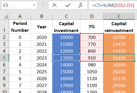
Here we will also use the formula for dynamic summation of cell values in the table. As seen below in the picture, to build a column with the future history of accumulation according to the exponential method, we need to add the obtained profit for each year and add it to the planned amounts of replenishment of the investment portfolio. Therefore, in cell E2, enter the following formula:

=C2+SUM($D$2:D2)

For a beautiful presentation, format the report with conditional formatting, a chart, and interactive Excel developer controls. The result exceeds the client's expectations:

Download

Now we can visually see how much and in what period the exponential method brings more profit compared to the traditional linear strategy. Thus, formulas and standard Excel tools allow us to quickly generate informative reports, presentations, creative materials, and other important documents for visualizing valuable information.