Get the second duplicate minimum or maximum value in Excel

When working with large tables, you often encounter repeating sum values in different rows. You might need to find only the first minimum value with the lowest sum in the table, excluding other possible duplicate sums.



How to Get the First Duplicate Minimum Value

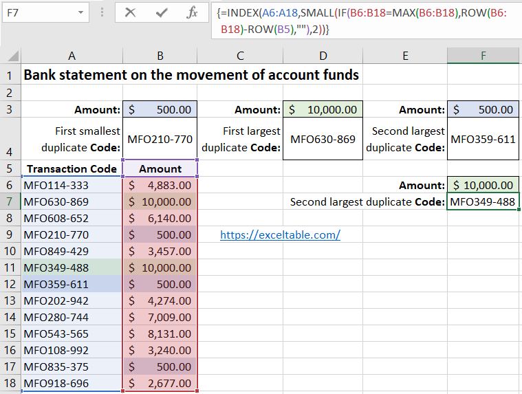
For demonstrating how to solve this problem, let's create a simple table:

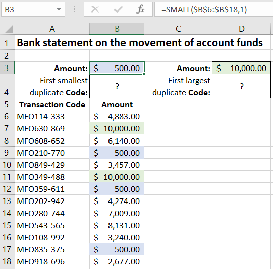
In this example, the data in question is in the range A6:B18. As you can see in the image, column A contains values, and column B contains their corresponding sums. Moreover, there are multiple minimum values scattered across different rows in column B.

To obtain the value from column A that corresponds to the first minimum sum in column B, follow these two simple steps:

1. In cell B4, enter the following formula:

=INDEX(A6:A18, MIN(IF(B6:B18=MIN(B6:B18), ROW(B6:B18)-ROW(B5), ""))

2. Confirm the formula entry by pressing CTRL+SHIFT+Enter since it needs to be executed as an array formula. If done correctly, you'll see curly braces {} appear in the formula bar.

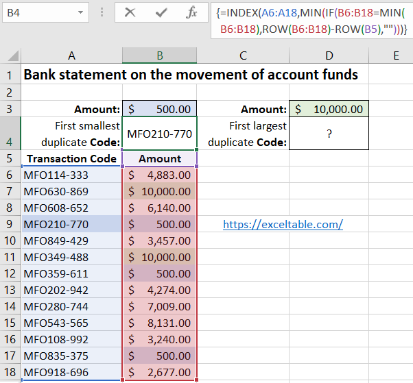
As a result, you'll obtain the value corresponding to the first minimum sum.

Detailed Explanation of the Formula for the First Minimum Value

The INDEX function is the most crucial part of this formula. Its nominal purpose is to look up a value in the specified table (range A6:A18 indicated in the first argument of the function) based on the coordinates provided in its second (row number of the table) and third (column number) arguments. Since the table used in the INDEX function only has one column A, the third argument is omitted (optional). In the meantime, multiple functions working with the range B6:B18 are used in the second argument of the formula.

In the first argument of the IF function, it tests if the value in each cell in the range B6:B18 is the minimum number. Thus, an array of logical values TRUE and FALSE is created in the program's memory. In this example, the array only contains three elements with a positive result of the test because the original table contains that many identical minimum values. If the result is positive, the formula proceeds to the next computational stage; if it's negative, the function returns an empty text value to the array in memory.

The next computational stage of the formula is to determine which row numbers contain these minimum sums. This step is essential to identify the first minimum value in the range B6:B18. It is accomplished with the ROW function, which creates another array in the program's memory, consisting of row numbers. Subtracting from these row numbers the number of the first row in the original table is crucial because the INDEX function doesn't work with row numbers in Excel but with row numbers of the table specified in its first argument. Therefore, to obtain the correct row number of the original table, you need to subtract the number of rows above the position of the table on the sheet from each row number. As a result, the program's memory will contain an array of row numbers. The MIN function then returns the smallest row number of the table that contains the minimum value. This number is used as the second argument for the INDEX function, which retrieves the value from the range A6:B18.

How to Get the First Duplicate Maximum Value

Now that we understand how the formula for the first minimum value works, we can modify it for our needs. For example, let's say we want to get the first maximum value. In cell D4, enter the modified formula:

=INDEX(A6:A18, MIN(IF(B6:B18=MAX(B6:B18), ROW(B6:B18)-ROW(B5), ""))

Don't forget to press CTRL+SHIFT+Enter to confirm the formula. This time, we simply replaced one of the MIN functions with MAX.

How to Get the Second Duplicate Minimum Value

To solve this task, enter a new modified formula in cell F3:

=INDEX(A6:A18, SMALL(IF(B6:B18=MIN(B6:B18), ROW(B6:B18)-ROW(B5), ""), 2))

To confirm the formula entry, press CTRL+SHIFT+Enter to execute it as an array formula. You'll immediately get the result:

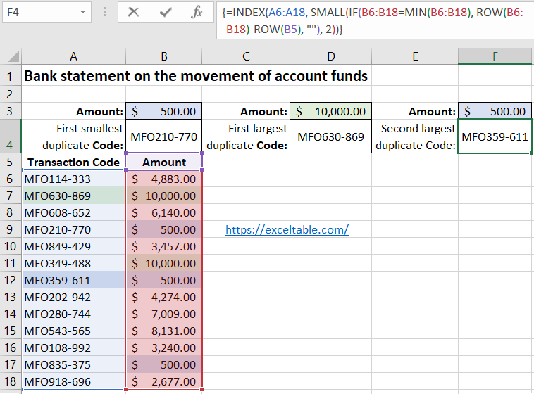
This time, we base this formula on the first one, but instead of using the MIN function, we utilize the SMALL function. The clever SMALL function is an improved version of MIN, allowing you to get the first, second, third, etc., minimum values. The order of the smallest values is specified in the second argument of the function. In this case, it's the number 2, so we get the second smallest row number from the array in the program's memory for the INDEX function.

How to Get the First Duplicate Maximum Value

To obtain the second maximum value, replace the MIN function with the MAX function in the formula:

=INDEX(A6:A18, SMALL(IF(B6:B18=MAX(B6:B18), ROW(B6:B18)-ROW(B5), ""), 2))

Download

Attention! If the number of duplicates in the range is less than the number in the second argument of the MIN or MAX function, these functions will return a "NUM!" error due to understandable reasons. Always clarify your goal before using the formula!