How to automatically change cell ranges in Excel
When working with data in Excel, it's often impossible to predict how much data will be collected in a particular table. This makes it challenging to define the exact range that a named cell should cover. The number of data points can change over time. To solve this issue, you can automatically adjust the named range of cells in Excel based on the amount of data.
How to Create Automatically Changing Ranges in Excel
Imagine you have an investment object, and you want to know the total profit over the period of its use. However, you can't predict the exact duration of its use. Yet, you need to constantly keep track of the total income from this investment object.
Create a profitability report for your investment object, as shown in the image below:
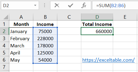
This task could be solved by summing an entire column B, and when new records are added, the total sum would update automatically. However, this is not the correct way to handle tasks in Excel. Firstly, you wouldn't be able to use cells in column B for entering other data. Secondly, continuously summing a whole column would consume more memory and could lead to issues in your document. The most efficient solution is to use dynamic named ranges.
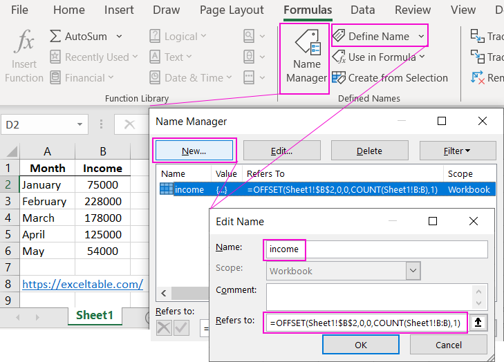
- Select "Formulas" > "Defined Names" > "Define Name".
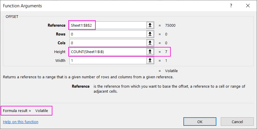
- Fill in the "Create Name" dialog box as shown in the image. Pay attention to the fact that in the "Refers to" field, we use the =OFFSET function, and one of its parameters involves the COUNT function. For example:
- Move the cursor to cell D2 and enter the formula =SUM with the name "income" as its parameter.
=OFFSET(Sheet1!$B$2,0,0,COUNT(Sheet1!$B:$B),1)
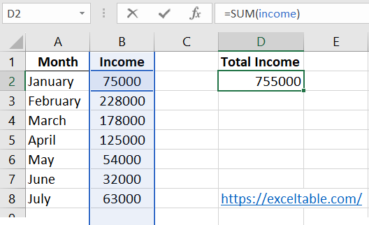
Now, as you gradually fill cells in column B, you can observe how the range covered by the "income" name changes automatically.
The OFFSET Function in Excel
Let's take a closer look at the functions we used when creating a dynamic name.
The function =OFFSET determines our range depending on the number of filled cells in column B. It has five parameters: =OFFSET(starting cell; row offset; column offset; height of the range; width of the range):
- "Starting cell" points to the upper-left cell from which the dynamic range will expand both downwards and to the right (if necessary).
- "Row offset" determines how many rows the range should be shifted vertically from the starting cell. These values can be zero or negative.
- "Column offset" specifies how many cells the range should be shifted horizontally from the starting cell. These values can also be zero or negative.
- "Height of the range" is the number of cells by which the range should increase in height. This parameter is self-explanatory.
- "Width of the range" is the number of cells by which the range should increase in width, starting from the initial cell.
The last two parameters are optional. If not filled, the range will consist of a single cell. For instance: =OFFSET(A1;0;0) refers to just cell A1, and =OFFSET(A1;2;0) points to A3.
Now let's examine the function =COUNT, which we included as the fourth parameter in the =OFFSET function:
What COUNT Function Determines
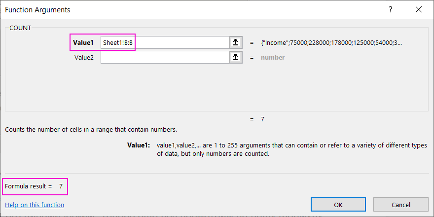
The function =COUNT($B:$B) automatically counts the number of filled cells in column B.
Therefore, by using the =COUNT() and =OFFSET() functions, we have automated the process of forming the range for the "income" name, making it dynamic. Now, let's revisit the formula we assigned the name "income" to:
=OFFSET(Sheet1!$B$2,0,0,COUNT(Sheet1!$B:$B),1)
Read this formula as follows: the first parameter indicates that our automatically changing range starts at cell B2. The next two parameters have values of 0;0, which means the dynamic range remains anchored to cell B2. The range expands only vertically, as indicated by the fourth parameter. This parameter contains the COUNT function, which returns the number of filled cells in column B. This means that the number of cells in the vertical range will be the value provided by the COUNT function. The final, fifth parameter sets the width of the range to 1.
Thanks to the COUNT function, we efficiently load into memory only the filled cells in column B, rather than the entire column. This fact eliminates potential memory-related errors when working with this document.
Dynamic Charts in Excel
Now that we have a dynamic name, let's create a dynamic chart for this type of report:
- Select the range B2:B6 and choose "Insert" > "Charts" > "2D-Column".
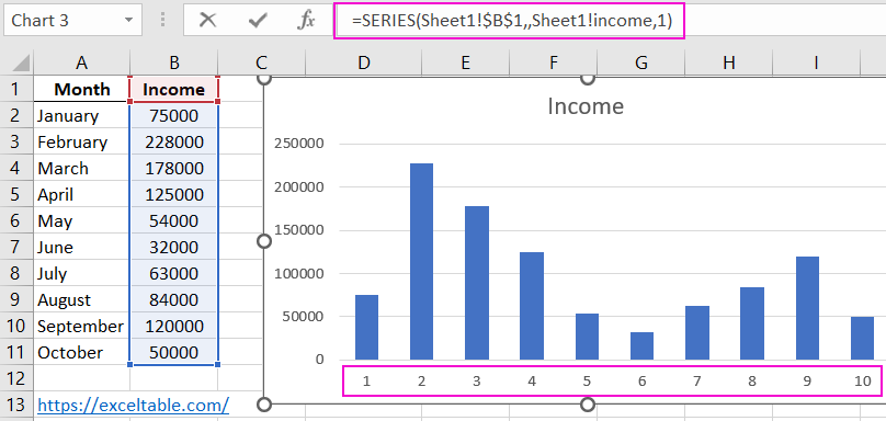
- Click on any column of the chart with the left mouse button, and the formula in the formula bar will display =SERIES().
- In the formula bar, change the parameters of the function from =SERIES(Sheet1!$B$1;;Sheet1!$B$2:$B$7;1) to:
- Add a new entry to the report in cells A8 ("July") and B8 ("63000"). Ensure that a new column is automatically added to the chart.
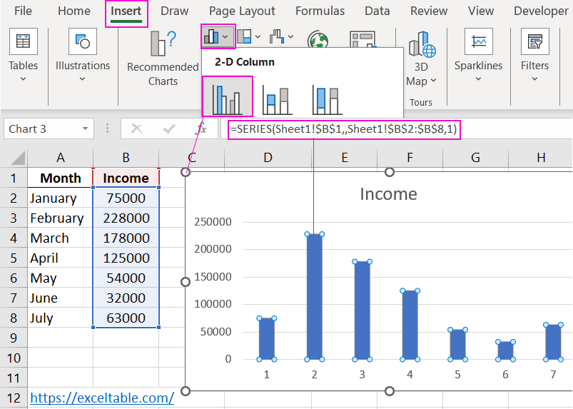
=SERIES(Sheet1!$B$1,,Sheet1!income,1)
 Download
Using our dynamic name "income," we managed to create an automatically changing dynamic chart that automatically adds and displays new data in the report.
