How to count and analyze Errors by code in Excel

Often, a complex situation arises when some formulas, instead of expected calculation results, display information about errors. A formula that can quickly find and count the number of erroneous values in tables with a large volume of data proves to be particularly useful. Sometimes, you just need to count errors in Excel as numerical values.

How to Count Errors in an Excel Formula

Before fixing errors in Excel, it's beneficial to provide Excel users with the ability to observe in real-time how many errors are left in the process of analyzing formula computation cycles. To achieve this, you need to count them all. Here is an example schematic table with formula errors:

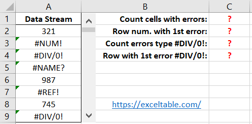
The image illustrates a problematic situation where some values in the table contain formula calculation errors in Excel where their results should be. To count the number of errors in the entire table, do the following:

In cell C1, enter the following formula:

=SUM(ISERR(A2:A9)*1)

This formula should be entered as an array, so after entering it, press the CTRL+SHIFT+Enter hotkey combination to confirm. If done correctly, curly brackets will appear in the formula bar.

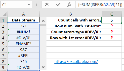
This way, you get the current number of errors in the table.

Formula breakdown for counting all errors in Excel cells:

Using the ISERR function, each cell in the range A2:A9 is checked for the presence of error values. The results of the function in the program's memory form an array of TRUE and FALSE logical values. After multiplying each logical value by the number 1, an array of 1s and 0s is obtained. Then, all elements of the array are summed, and the formula returns the count of errors.

How to Find the First Error in an Excel Value

For analyzing computational cycles, it is useful for the user to know not only the current number of uncorrected errors but also the row that contains the first error. To find the row where the first error occurs, use another formula:

=MIN(IF(ISERROR(A2:A9),ROW(A2:A9)))

Again, this formula should be entered as an array, so press CTRL+SHIFT+Enter to confirm.

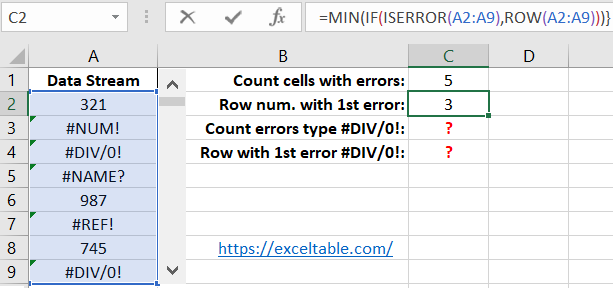
The first error is in the third row of the Excel worksheet.

Let's look at how this formula works:

Similar to the first formula, the ISERR function creates an array of TRUE and FALSE logical values in the program's memory. Then, the ROW function returns the current row numbers of the cells in the range A2:A9. Using the IF function, in the array with TRUE and FALSE logical values, TRUE is replaced with the current row number. Afterward, the MIN function selects the smallest number from this array.

How to Count Excel Errors with a Specific Code

Another useful piece of information for a user engaged in error checking is the count of a specific type of error. To obtain such a result, use the third formula:

=COUNTIF(A2:A9,"#DIV/0!")

This time, the formula should not be entered as an array, so simply press Enter after inputting it to confirm.

The third formula returns the count of division by 0 errors (#DIV/0!). However, it works equally effectively if you specify another type of error in the second argument of the COUNTIF function in Excel cells. For example, #NAME?

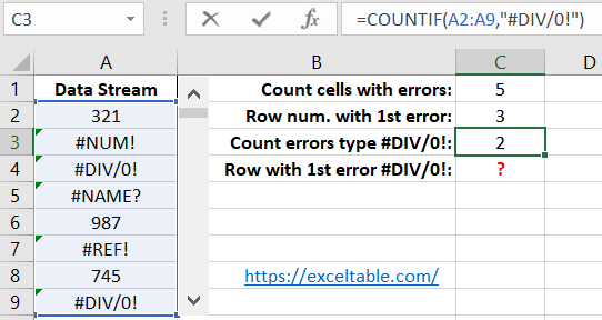
As seen in the image, everything works just as effectively.

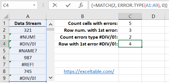
To find in which row the first error of a specific type and code occurs, use the fourth formula:

=MATCH(2, ERROR.TYPE(A1:A9), 0)

As shown in the next image, the formula returns the value 4, which corresponds to the row number where the division by 0 error first occurs.

Excel Error Codes and Types

download file Download

The ERROR.TYPE function checks each cell in the range A1:A9. If it encounters an error, it returns its corresponding number (e.g., the error code for division by zero: for the #DIV/0! type, it is code 2). Below is an entire table of types and codes for handling Excel errors:

Type	Code
#NULL!	1
#DIV/0!	2
#VALUE!	3
#REF!	4
#NAME?	5
#NUM!	6
#N/A	7
#GETTING_DATA	8
#SPILL!	9
#CONNECT!	10
#BLOCKED!	11
#UNKNOWN!	12
#FIELD!	13
#CALC!	14

Next, an array of values with error code numbers is created in the program's memory. In the first argument of the MATCH function, we specify the error code we need to find. In the third argument, we specify the code 0 for the MATCH function, meaning that it should return the first encountered value of 2 in the array if duplicates are present.

Attention! In the fourth formula, we referred to the range of cells starting from A1 and ending at A9. This is because the MATCH function returns the current position of the value relative to the table, not the entire sheet. Therefore, in the second argument of the MATCH function, the range of values to be searched should be specified so that the position numbers match the row numbers on the sheet. In other words, if we had specified the address range A2:A9, the formula would have returned the value 5, which is incorrect.