How to create a case-insensitive Excel formula for searchin
Functions like VLOOKUP and similar search functions have a limitation - they cannot differentiate between uppercase and lowercase characters. This limitation can be quite frustrating and, at times, significantly complicating for certain tasks in Excel. If your Excel task requires considering the case sensitivity in text values, you can replace the VLOOKUP (or similar) function with a formula.
How to Make Excel Formulas Case Sensitive
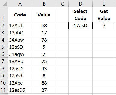
Let's assume that the content of the original value you want to search for is in cell D1, and the table to search within is in the range A1:B11.
To find the required values, follow these steps:
- In cell E1, enter the following formula:
- After entering the formula, press the keyboard shortcut CTRL+SHIFT+Enter to confirm it, as the formula should be executed as an array. If done correctly, you will see curly braces { } appear in the formula bar.
=IF(OR(EXACT(A1:A11,D2)),INDEX(B1:B11,MAX(EXACT(A1:B11,D2)*ROW(A1:B11)),"")
The example table and the formula in action are shown in the image below:
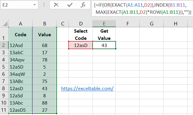
As you can see, the search criteria now take case sensitivity into account.
 Download
Attention! If the table does not contain the original value for the search, the formula will return an empty cell. If the table contains multiple duplicates of the original value, the formula will return the last duplicate. This is in contrast to the VLOOKUP function, which returns the first duplicate if duplicates are present.
How the Case Sensitive Search Formula Works
The formula uses the =EXACT() function to find values by comparing two texts. It takes case sensitivity into account and returns TRUE if the text values match exactly, and FALSE otherwise. Since we use this function in an array formula, it compares the value in D1 with each value in the cells of the table in the range A1:A11.
The role of the =IF() function is to return an empty text when the logical expression OR(EXACT(A1:A11,D1)) returns FALSE. The formula will return an empty text if the EXACT function doesn't find any matches when comparing with the original text. If it finds a match, the formula performs a secondary search within the fragment of the formula: EXACT(A1:A11,D1)*ROW(A1:B11). This will find the row number that contains the matching value. Here, we utilize the fact that logical values TRUE and FALSE are converted to numbers 1 and 0 during arithmetic operations. If the text is found during the search, it returns a value corresponding to the row number (otherwise it's equal to 0). The =MAX() function selects the highest of the row numbers and passes it as an argument to the =INDEX() function, which ultimately returns the final result by displaying the cell value from column B for the selected row number.
