How to Create Dependent Dropdown Lists in Excel Step by Step

A dependent dropdown list unveils a trick often praised by Excel template users. It's a trick that makes your work easier and faster, ensuring your forms are convenient and pleasant.

Example of Creating a Dependent Dropdown List in an Excel Cell

Explore the use of a dependent dropdown list in crafting a user-friendly document form for product ordering by sellers. From the entire range, they had to choose the products they intended to sell.

Each seller first identified the product group and then a specific item from that group. The form needed to include the full name of the group and a specific product index. Since manually typing this would be too time-consuming (and annoying), I proposed a very quick and simple solution - 2 dependent dropdown lists.

The first was a list of all product categories, and the second was a list of all products within the selected category. Thus, I created a dropdown list dependent on the choice made in the previous list (you can find material on creating two dependent dropdown lists here).

A user of a home budget template also wants the same result, where both category and subcategory of expenses are needed. An example of the data is shown in the image below:

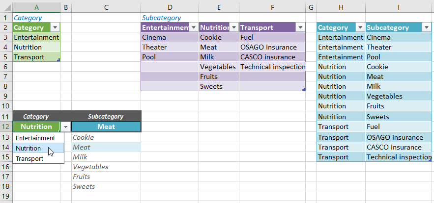
For instance, if we choose the Entertainment category, the subcategory list should include: Cinema, Theater, Pool. It's a rapid solution if you want to analyze more detailed information in your home budget.

List of Categories and Subcategories in a Dependent Excel Dropdown List

I admit that in my proposed version of a home budget, I limit myself to just the category because, for me, this division of expenses is sufficient (expense/income names are considered subcategories). However, if you need to divide them into subcategories, the method I describe below will be perfect. Go ahead and use it!

The final result looks like this:

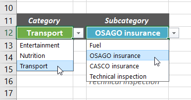
Dependent Dropdown List of Subcategories

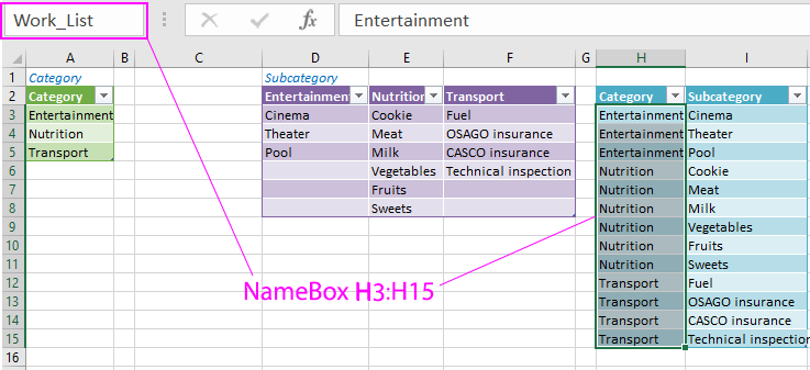
To achieve this, you need to create a slightly different data table than if you were creating a single dropdown list. The table should look like this (range H2:I15):

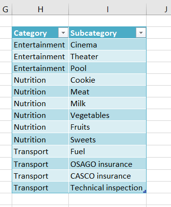
Excel Original Working Table

In this table, enter the category and its subcategories next to it. The category name should be repeated as many times as there are subcategories. It's crucial that the data is sorted by the Category column. This will be extremely important when we write the formula later.

You could also use tables from the first image. Of course, the formulas would be different. Once I even found a solution online, but I didn't like it because there was a fixed length of the list: sometimes it contained empty fields, and sometimes it didn't display all the elements. Of course, I could overcome this limitation, but I confess that I prefer my solution, so I never returned to that one.

Okay, great. Now, step by step, I'll describe the process of creating a dependent dropdown list.

1. Cell Range Names

This is an optional step; you can easily manage without it. However, I like to use names because they significantly facilitate both writing and reading the formula.

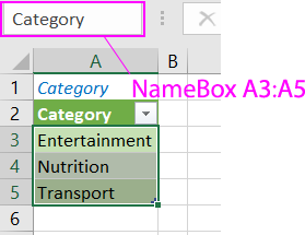
Assign names to two ranges: the list of all categories and the working category list. These will be ranges A3:A5 (category list in the green table in the first image) and H3:H15 (repeating category list in the purple working table).

To name the category list:

Select the range A3:A5.
In the name field (left of the formula bar), enter the name "Category."
Confirm with the Enter key.

Perform the same action for the range of the working category list G3:G15, which you can call "Work_List." This range will be used in the formula.

2. Creating a Dropdown List for Category

It's simple:

Select the cell where you want to place the list. In my case, it's A12.
In the "DATA" menu, choose the "Data Validation" tool. The "Data Validation" window will appear.
Choose "List" as the data type.
As the source, enter: =Category (see the image below).
Confirm with OK.

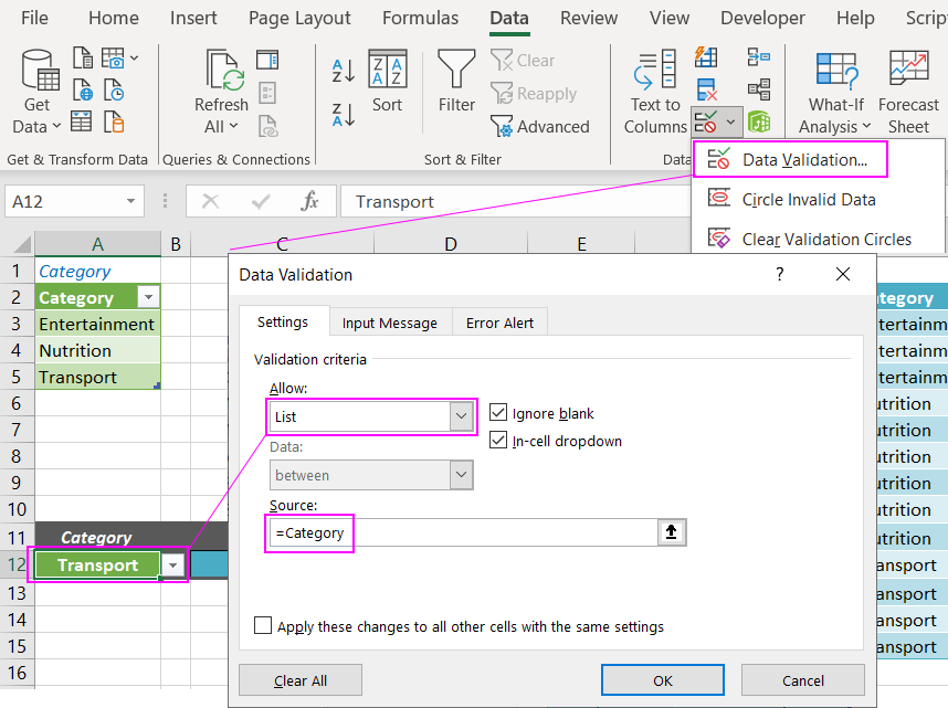
Data Validation – Category.

The result is as follows:

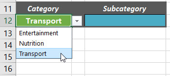
Dropdown list for the category.

3. Creating a Dependent Dropdown List for Subcategory

Now it gets fun. We know how to create lists - we just did it for the category. The only question is, "How do we tell Excel to select only those values that are intended for a specific category?" As you probably guessed, I will use the working table and, of course, formulas here.

Let's start with what we already know, i.e., creating a dropdown list in cell B12. So, select this cell and click "Data" / "Data Validation," choosing "List" as the data type.

In the list source, enter the following formula:

=OFFSET($I$2,MATCH(A12,Work_List,0),0,COUNTIF(Work_List,A12),1)

View of the "Data Validation" window:

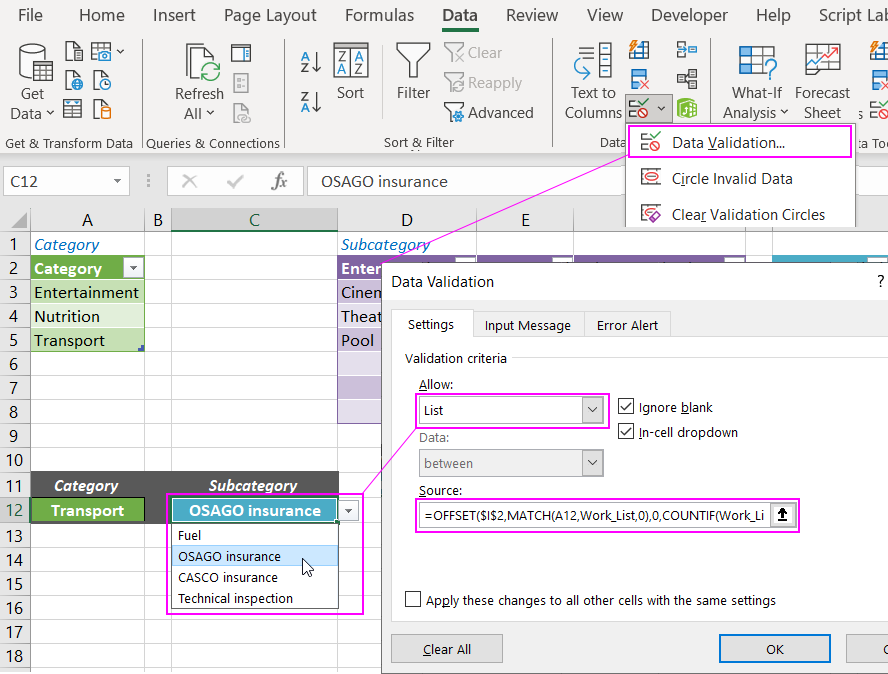
Data Validation for Subcategory in the Dependent Dropdown List

As you can see, the entire trick of the dependent list lies in using the OFFSET function. Well, almost the entire trick. It is aided by the SEARCH and COUNTIF functions. The OFFSET function allows dynamically determining ranges. Initially, we determine the cell from which the range shift should begin, and in the subsequent arguments, we define its dimensions.

In our example, the range will move along the Subcategory column in the working table (H2:I15). We start the shift from cell H2, which is also the first argument of our OFFSET function. In the formula, we wrote cell H2 as an absolute reference because I assume we will use the dropdown list in many cells.

Since the working table is sorted by Category, the range that should be the source for the dropdown list will start where the selected category first appears. For example, for the Food category, we want to display the range H6:H11; for Transport - the range H12:H15, and so on. Note that we are always moving along column H, and the only thing that changes is the start of the range and its height (i.e., the number of items in the list).

The start of the range will be shifted relative to cell H2 by the number of cells down (by the number) equal to the position number of the first occurrence of the selected category in the Category column. It will be easier to understand with an example: the range for the Food category is shifted 4 cells down relative to cell H2 (starts 4 cells from H2). In the 4th cell of the Subcategory column (excluding the header, as it is about the range named Work_List), there is the word Food (its first appearance). We use this fact to determine the start of the range. We use the SEARCH function for this purpose (entered as the second argument of the OFFSET function):

MATCH(A12,Work_List,0)

The height of the range is determined by the COUNTIF function. It counts all occurrences in the category, i.e., the word Food. The number of times this word appears is the number of positions in our range. Here is the function:

COUNTIF(Work_List,A12)

Of course, both functions are already included in the OFFSET function described above. Also, note that both in the SEARCH and COUNTIF functions, there is a reference to the range named Work_List. As I mentioned earlier, it is not necessary to use range names in the formula; you can simply enter $H3: $H15. However, using range names in the formula makes it simpler and easily readable.

That's all:

download file Download

One formula, not so simple, but it makes the work easier and protects against data entry errors!

I've presented two ways to use this trick. I wonder how you will use it?