How to Create an ID Number Generator Using Excel Formula

Very often, data entered in Excel spreadsheets is used to populate database files. Files of this type often require compliance with filling rules, such as ensuring that certain data fields have a specific length of characters. Therefore, the technique of populating data fields with numerical values often requires the addition of extra zeros to ensure that all values have the same number of characters regardless of the numeric magnitude.



Automatically Adding Characters to an Excel Cell

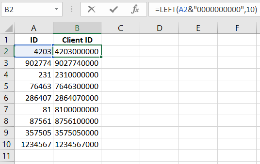
In Excel, preparing and populating data with additional zeros is a fairly straightforward method. For example, if each value in the "Customer ID" field should have 10 digits, to achieve this, the corresponding number of zeros needs to be added to each number. For instance, for the identifier with the number 1234567, three zeros need to be added, resulting in the correct entry of 1234567000 for the "Customer ID" field in the database file.

The image below demonstrates the automatic filling of the missing number of characters with zeros at the end of the string using a simple formula:

or like this:

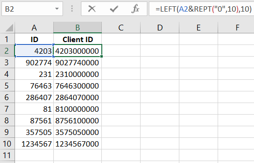
As a result, each identifier now has the necessary number of zeros to comply with the rule for further filling the "Customer ID" field when importing the table into the database.

The formula shown in the image above first adds a series of 10 zeros to the value of cell A4, resulting in a new identifier. Each of them now has at least 10 digits in any case.

Then, the LEFT function is applied, which trims each original value to the first 10 digits from the beginning of the string. For this, the second argument of the LEFT function is specified as the number 10.

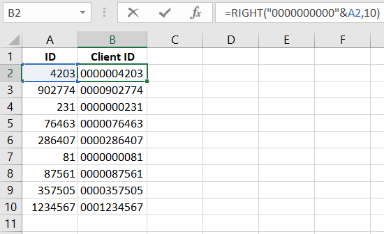
If you need to automatically add zeros not from the right side but from the left (for example, like this: 0001234567), then you should slightly modify the formula and use the RIGHT function instead of the LEFT:

Download

Now you can perform various combinations with identifiers for your formulas.

As seen in the image, this time, using the ampersand symbol, we added 10 zeros to the left of the original value in cell A4. Then, we trimmed each identifier, leaving only 10 numeric digits on the right side of the numbers. We added the missing characters from the beginning of the required string. This is how the RIGHT function works, in inverse proportion to the previous LEFT function.