How to find a value in an Excel table by column and row
In the Excel table, a database from the sales report for the first half of the year is loaded. We need to extract values from the database based on multiple conditions. It's important to note that during the extraction, the search criteria will be perpendicular. Initially, we'll perform a vertical lookup separately for the column range, and then a horizontal lookup for values across the row range. Such a relational query cannot be implemented using the INDEX function. In this example, let's explore the new capabilities of Excel formulas.
Search for Values in Excel Table
To solve this problem, let's illustrate an example on a schematic table that corresponds to the conditions described above.
Sheet with a table for searching values vertically and horizontally:
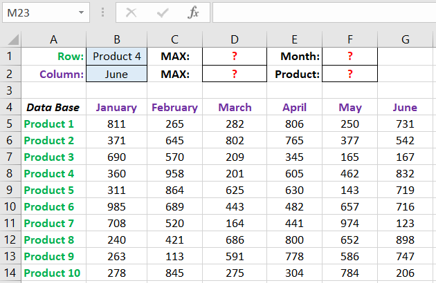
Above the table is a row of results. In cell B1, enter the criterion for the search query, i.e., the column header or row name. And in cell D1, the search formula should return the result of calculating the corresponding value. After that, in cell F1, the second formula will work, which will use the values of cells B1 and D1 as criteria to search for the corresponding month.
Search for Value in Excel Row
Now let's find out the maximum volume and in which month the maximum sales of Product 4 occurred.
To search by columns, follow these steps:
- In cell B1, enter the value of Product4 – the row name, which will serve as the criterion.
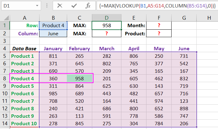
- In cell D1, enter the following formula:
- To confirm after entering the formula, press the keyboard shortcut CTRL+SHIFT+Enter, as the formula must be executed in an array. If done correctly, curly braces will appear in the formula bar.
- In cell F1, enter the second formula:
- Again, press CTRL+SHIFT+Enter to confirm.
=MAX(VLOOKUP(B1,A5:G14,COLUMN(B5:G14),0))
=INDEX(B4:G4,1,MATCH(D1,VLOOKUP(B1,A5:G14,COLUMN(B5:G14),0),0))
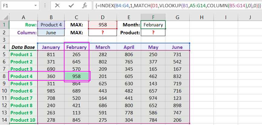
Found in which month and what was the highest sales of Product4 over two quarters.
Search for Value in Excel Column
The second option of the task will be to search the table using the month name as a criterion. In such cases, we need to modify the skeleton of our formula: replace the VLOOKUP function with HLOOKUP, and replace the COLUMN function with ROW.
This will allow us to find out the volume and which product had the maximum sales in a specific month.
To find which product had the maximum sales volume in a specific month, follow these steps:
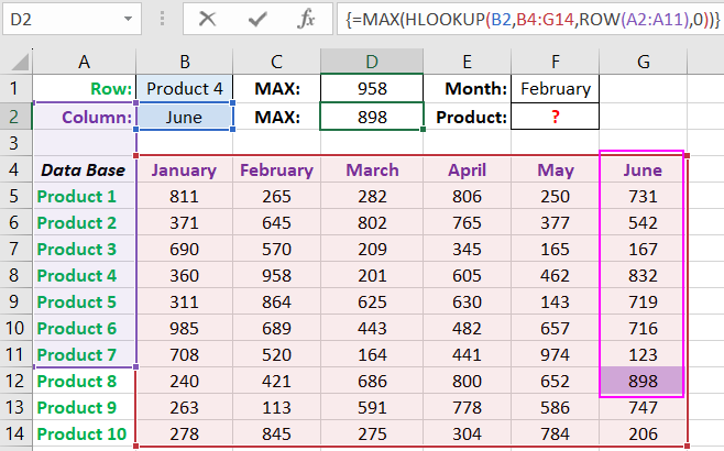
- In cell B2, enter the month name June – this value will be used as the search criterion.
- In cell D2, enter the formula:
- To confirm after entering the formula, press the keyboard shortcut CTRL+SHIFT+Enter, as the formula must be executed in an array. And curly braces will appear in the formula bar.
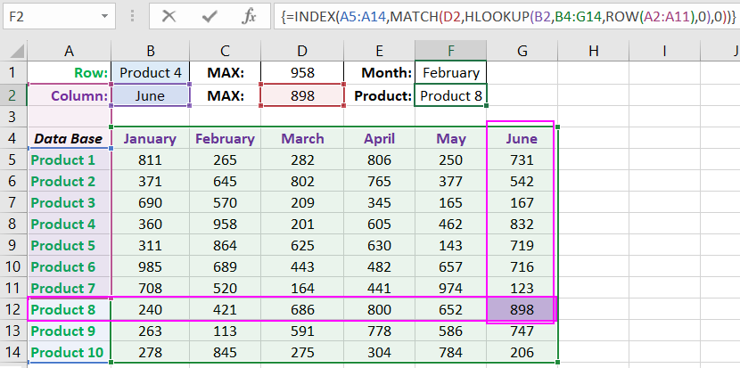
- In cell F1, enter the second formula:
- Again, press CTRL+SHIFT+Enter to confirm.
=MAX(HLOOKUP(B2,B4:G14,ROW(A2:A11),0))
=INDEX(A5:A14,MATCH(D2,HLOOKUP(B2,B4:G14,ROW(A2:A11),0),0))
Operating principle of the Excel column search formula:
 Download
In the first argument of the HLOOKUP function (Horizontal Lookup), specify the reference to the cell with the search criterion. In the second argument, the reference to the range of the table being viewed is specified. The third argument generates the ROW function, which creates an array of row numbers in memory with 10 elements. Since there are 10 rows in the table part.
