How to Round Decimal and Integer Numbers in Excel

Clients of every company usually prefer to see simple rounded numbers. Reports with fractional numbers beyond tenths or hundredths, which do not affect accuracy significantly, are much less readable. Therefore, in Excel, it is necessary to use the ROUND function for numerical rounding values, as well as its modifications such as ROUNDUP(), ROUNDDOWN(), and others.



How to Round Decimal and Integer Numbers in Excel?

The ROUND function in Excel is used to round the original numerical value to a specified number of digits (decimal places or precision) after the decimal point. The function has only 2 arguments:

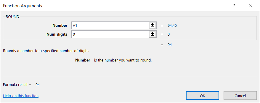
1. Number – specifies the original number to be rounded or a reference to the cell containing it.
2. Number_digits – specifies the number of decimal places to leave after the decimal point.

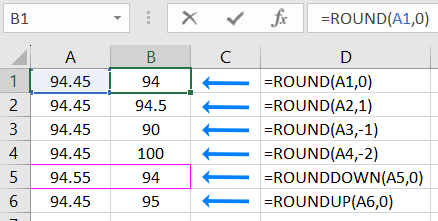
If you specify the number 0 in the second argument of the ROUND function, Excel will remove all decimal places and round the original numerical value to the nearest integer based on the first digit after the decimal point. For example, with an original value of 94.45, the function returns the integer 94, as in cell B1.

Next, let's look at examples of how to round integers in Excel. This technique is often needed in presentations of analyses of various indicators.

How to Round a Number to Hundreds of Thousands in Excel?

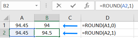
If you specify the number 1 in the second argument, Excel will round the original value to one decimal place after the decimal point based on the second numerical value after the decimal point. For example, if the original value is 94.45, then the ROUND function with 1 in the second argument returns the fractional value to the tenths place, 94.5. Cell B2:

In the second argument for the ROUND function, you can also use negative numerical values. Thanks to this method, Excel rounds the number based on the digits to the left of the decimal point, i.e., on the left by 1 digit. For example, the following formula with a negative number -1 in the second argument returns the numerical value 90 for the same original number 94.45:

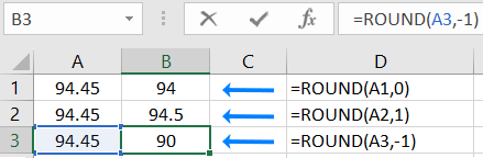
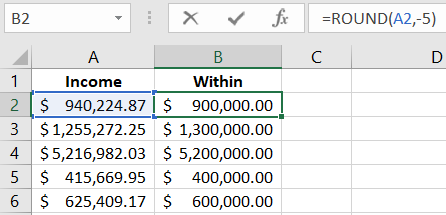
Thus, we have rounded not only to the nearest integer but also to the tens place. Now it's not difficult to guess how to round an integer in Excel to the hundreds of thousands. To do this, in the second argument, simply specify a negative value -5, since there are 5 zeros in the hundreds of thousands (5 digits to the left of the decimal point). Example:

Example of a formula with practical application of the ROUND function

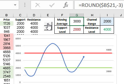
The data visualization developer in Excel has received another Technical Task from management to create visual analyses and reports. Dynamic Excel charts need to display changes in stock prices between support and resistance levels, which dynamically shift as soon as the price breaks through them:

1. If support is breached, the levels shift downward.
2. If the price breaks through resistance, the levels shift upward.
3. If the price makes minor changes within the range channel between support and resistance, the levels remain unchanged.
4. The channel range between levels should be able to change based on user-defined values (cell I1).

First, let's calculate a simple moving average based on the magnitude of the channel range between support and resistance levels. To do this, we'll use the rounding formula to the nearest thousand, as stock price quotes are traded in thousands as of the selected analysis period. In cell G1, enter the formula:

=ROUND($B$21,-3)

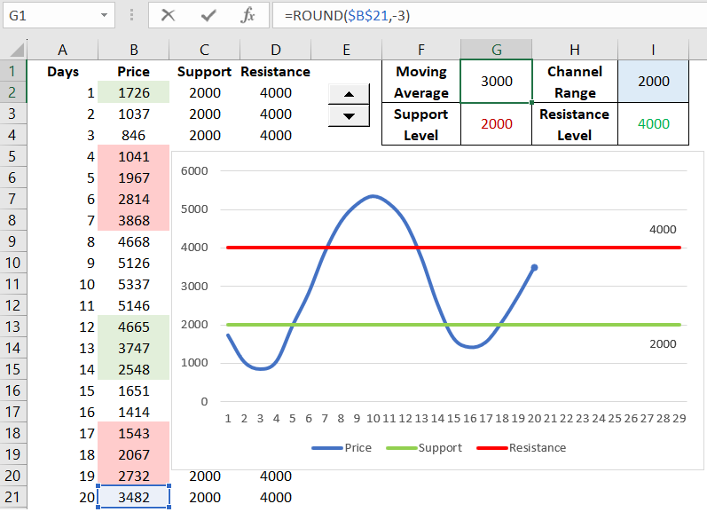
1. The first argument of the formula refers to the $B$21 link to the last updated stock price.
2. In the second argument of the ROUND function, a negative value of -3 is used to round to the nearest thousand.
3. In cell G3, we calculate the support level based on the values obtained in G1 and the user-specified range magnitude in cell I1. We simply divide the range in half and subtract the difference from the moving average to get the support level:

=G1-I1/2

4. In cell I3, to get the resistance level, we similarly divide the range in half, but this time we don't subtract the difference; instead, we add it to the MA value:

=G1+I1/2

As a result, we get a dynamic chart in Excel.

Download

This is one of many examples where it's very useful to use the ROUND function with negative values in the second argument in formulas. We will use this trick many times in our Excel examples.

How to Round to Whole Numbers Up or Down?

With the ROUNDUP and ROUNDDOWN functions, you can force Excel to round in the required direction. These functions allow you to work against rounding rules. For example:

The ROUNDUP function rounds up. Suppose the original value is 94.45; then ROUNDUP in the desired rounding direction upwards returns 95:

=ROUNDUP(94.45,0) = 95

The ROUNDDOWN function rounds another original numerical value, 94.55, and returns 94:

=ROUNDDOWN(94.55,0) = 94

Attention! If you use rounded numbers in cells for further use in formulas and calculations, then be sure to use the ROUND function (or its modifications) and not cell formatting. Because cell formatting does not change the numerical value, it only changes its display.

As seen in the screenshot, the true numerical value of the cell is displayed in the formula row without formatting. Therefore, cell formatting does not round the number, and as a result, serious errors in calculations may occur.