How to round to significant figures using Excel formula

In some financial reports, indicator data is presented with precision rounded to specific significant figures. What does significant figure mean? The point is that in the visual analysis of reports presentations with millions, there is no need to clutter up with exact numerical values, displaying every digit in the number (units, tens, hundreds, and thousands), to avoid compromising the readability of the data.

For example, instead of specifying the amount of $883,788 in the report presentation, it can be rounded to one significant figure. This means that after rounding, the amount easy to perceive will be displayed as $900,000. If you round the original number to two significant figures, the resulting value will be $880,000.



How to Round to Three Significant Figures in Excel

In Excel, the user has control. The program will round fractional or even whole numbers depending on the number of significant figures that satisfy the user's needs. Undoubtedly, at first glance, such rounding may raise doubts about the rationality of the decision. However, presentations accommodate both precise and relative indicators. In other situations, it is also applicable. For example, in strategic planning, more important are relative indicators, as no matter how much you plan, you will never guess exact resulting numbers. In tactical planning, precise values are more important to avoid serious miscalculations. In strategic planning, where indicators reach millions, any value below a certain number of significant figures is insignificant.

Below is a figure showing how to create a formula that rounds millionth numerical values to a specified number of significant figures:

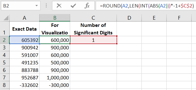
The ROUND function is used to round the original numerical value to a certain number of decimal places. The function contains 2 arguments:

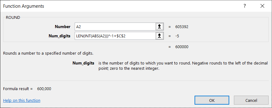
1. Number - a reference to the original value to be rounded.
2. Num_digits - the number of digits to leave after rounding the original number.

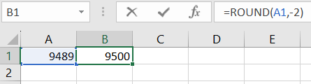
If a negative number is specified in the second argument of the ROUND function, Excel will round the original numerical value according to the digits to the left of the decimal point. For example, the following formula returns the result of the calculation as 9500:

And if you specify -3 in the second argument, then the ROUND function returns the result as 9000:

This formula works well, but not always. For example, what if the original numerical values are in different numerical ranges? Some are over a million, while others barely exceed hundreds of thousands. If there is a need to round all such original values to the same significant figure using the same formula (as is usually done in Excel). Applying the ROUND function with different values in the arguments for separate groups of original values is not the right, or more precisely, not the best solution. Although theoretically, everything might work.

For a neat solution to this problem, a constant immutable number of significant figures should be used in the formula that will calculate the corresponding values.

How to Determine the Number of Significant Figures in Excel

Suppose the original value is the number -2330.45. To calculate the number of significant figures in the ROUND function, you can use the following formula:

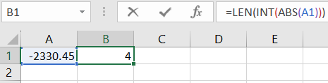
This formula first converts the given negative original number to a positive one using the ABS function (removes the minus sign from the front if present). The obtained result is then processed by the INT function, which removes all decimal places. Then, the resulting result is processed by the LEN function to count the number of characters in the original numerical value without the minus sign and decimal point.

In this case, the LEN function returns the value 4. If we remove the minus sign and the numbers after the decimal point from the number -2330.45, we get 4 digits.

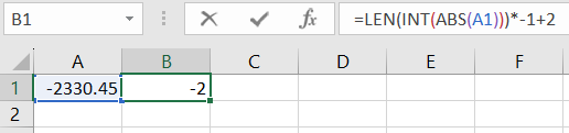
Next, the result of the function is multiplied by the negative number -1 to obtain a negative value (for the second argument of the ROUND function). After that, the desired number of significant figures is added. In this example, the calculation looks like this: 4*(-1)+2=-2.

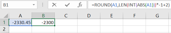
Like in the previous examples, this formula will be used as the second argument for the ROUND function. Enter the following formula in Excel and round the original data -2330.45 to -2300:

Rounding to 3 Significant Figures in Excel

The number 2 specified in the argument of this formula can be replaced with a reference to a cell where the user will specify the desired number of significant figures. As shown in the picture with the first example.

This way, you can round to 3 or 5 significant figures. Just specify the desired value in cell C2.

Practical Application of Rounding Formulas to Significant Numbers

Rounding to the nearest significant values in Excel can be done with a choice of direction: to the nearest smaller or larger round number. To do this, use formulas with the FLOOR.MATH and CEILING.MATH functions.

Let's give an example of the practical application of the formula for rounding original values to significant round numbers using the FLOOR.MATH function. For this, as always, we simulate the situation.

Round Levels Trading Strategy

For the Excel data visualization developer, a new Technical Task has been received. There is a simple but very effective trading strategy based on round levels. The foundation of this strategy lies in the fact of market psychology – traders tend to open buy or sell orders at round prices, or close to them. Also, stop orders. As a result of the large accumulation of orders at round prices, financial asset values often form quite strong support or resistance levels. These are commonly referred to as Round Levels.

Key principles of trading using the round levels strategy:

1. Analysis should be conducted in the area of round prices. Traders find it easier to perceive round numerical values. They require less attention to concentration, memory, analysis, reduce the risk of human error or technical error, etc.
2. It is essential to observe financial safety measures. When the price approaches round levels, market volatility often increases.
3. It is always important to remember that the round levels trading strategy is not a universal solution for a trader. Its effectiveness can vary significantly depending on market conditions at certain times.

One cannot trade a strategy without preliminary analysis. The Excel data visualization developer must create a chart that will automatically set round levels. The range of levels should have an expansion or contraction function. So that traders can adjust the conditions depending on the market price volatility of the financial asset.

To solve this task, the developer uses the formula:

=FLOOR.MATH(B3,$C$1)

where:

1. The first argument specifies the relative reference to the cell with the first original price.
2. The second argument specifies the absolute reference to the cell with the significant numerical value to which the original price should be rounded down – this will be the support level.
3. The second argument also serves as the size of the range set between the round levels.
4. The support round level values plus the range width together form the resistance level.

The result of data visualization for the trading strategy analysis – Round Levels:

Download

Using the INDEX formula in the range of original chart cells (B3:B22), prices from the market history are filled in. In cell $C$1, the trader specifies the range of expansion between support and resistance levels. This allows finding the optimal range size for a specific price volatility. And all this can be very easily implemented in MS Excel using standard formulas without programming. To make sure of this, download the ready-made template via the link under the image.