How to split text into multiple cells in Excel
Oftentimes, it's necessary to optimize the data structure after importing it into Excel. Various values end up in a single cell, forming an entire string as one value. The question arises: how to split a string into cells in Excel. The program offers various search functions; some search by cells, while others search by the content of cells. Searching within a text string contained in a cell is also a common need for Excel users. We will use these functions to split strings.
How to Split Text into Two Excel Cells
Suppose data has been imported into an Excel sheet from another program. Due to data structure incompatibility during import, some values from different categories have been entered into a single cell. It is necessary to separate whole numerical values from this cell. An example of such incorrectly imported data is shown below:
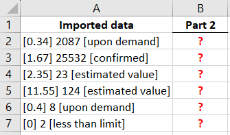
First, let's determine the pattern by which we can identify that data from different categories, despite being in the same row. In our case, we are only interested in numbers outside square brackets. What effective way can we quickly select entire numbers from strings and place them in separate cells? The solution is an adaptable formula based on text functions.
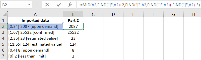
Enter the following formula into cell B3:
=MID(A2, FIND("]", A2) + 2, FIND("[", A2, FIND("]", A2)) - FIND("]", A2) - 3)
Now copy this formula along the entire column:
Selection of numbers from strings into separate cells.
Description of the formula for splitting text into cells
 Download
The MID function returns a text value containing a specific number of characters in a string. The arguments of the function are:
- The first argument is a reference to the cell with the original text.
- The second argument is the position of the first character from which the split string should start.
- The last argument is the number of characters that the split string should contain.
The first argument of MID is clear – it is a reference to cell A3. We calculate the second argument with the help of the FIND function("]", A3) + 2. It returns the next number of the character after the space following the closing square bracket. In the last argument, the function calculates how many characters the split string will contain after the separation, taking into account the position of the square bracket.
Note! In our example, the original and split strings have different lengths and different numbers of characters. This is why we called such a formula flexible at the beginning of the article. It is suitable for any conditions when solving such problems. The flexibility is provided by a complex combination of FIND functions. The formula user only needs to determine the pattern and specify it in the parameters of the functions: whether it's square brackets or other separating signs. For example, it could be spaces if you need to split a string into words, etc.
In this example, the FIND function, in the second argument, determines the position relative to the first closing bracket. And in the third argument, the same function calculates the position of the text we need in the string relative to the second opening square bracket. The calculation in the third argument is more complex and involves subtracting the length of the larger text from the smaller one. To account for 2 additional spaces, subtract the number 3. As a result, we get the correct number of characters in the split string. With such a flexible formula, you can extract split text of different lengths from strings of different lengths.
