How to use 3D References in Excel Formulas Exaples
Best practices for using 3D references in Excel formulas, when a formula refers to another sheet or workbook, it is considered a three-dimensional reference.
Most Excel users primarily work with formulas that process data on the same sheet where the formula resides, for example, like =B32 or =AV123. In such cases, the cell addresses and formulas exist in a two-dimensional plane, making them two-dimensional references.
When you extend the reference address beyond the boundaries of the current sheet (e.g., =Sheet2!B32), it allows you to work in a three-dimensional space of cells. Let's explore specific examples.
Practice using Three-Dimensional References in Excel
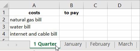
Start by creating a new workbook with four sheets: "1 Quarter," "January," "February," and "March." In each sheet, enter the same values in cells A1:A4: "costs," "natural gas bill," "water bill," "internet and cable bill."
In cells B2:B4 of each month's sheet, enter different amounts corresponding to the month's expenses. Format the cell values as currency.
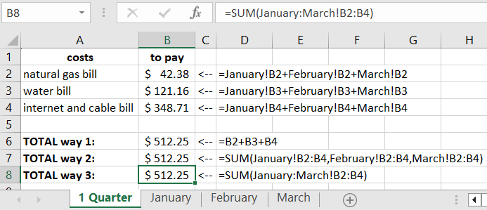
In the "1 Quarter" sheet, enter three-dimensional formulas in cells B2:B4 to sum the amounts for each month according to the expense type. In cell B6, calculate the total expense amount using a two-dimensional formula.
Entering a three-dimensional formula. Method 1:
- Go to the "1 Quarter" sheet, select cell B2, and enter the equal sign "=",
- Click on the "January" sheet's tab to navigate there. Click on cell B2 and type the plus sign "+" using your keyboard. At this point, the formula should display the reference as shown below:
- Repeat the previous step for the "February" and "March" sheets (no plus sign is needed after "March"), then press Enter.
- Once the formula is fully entered, press the Enter key.
- Copy the formula from cell B2 on the first sheet to cells B3:B4.
- In cell B6, sum the expenses in the range B2:B4 using regular addition: =B2+B3+B4.
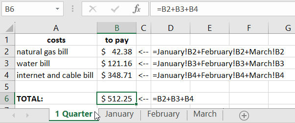
You can initially enter a three-dimensional formula in cell B2 on the "1 Quarter" sheet manually by typing the sheet names:
=January!B2+February!B2+March!B2
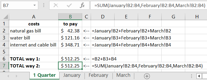
Method 2: You can use the SUM() function in the formula, specifying references to non-adjacent ranges on different sheets. For example:
=SUM(January!B2:B4,February!B2:B4,March!B2:B4)
Method 3: You can use a shortened version of the SUM() function's arguments by specifying three-dimensional ranges. Look at the formula in cell B8 in the image. Example:
=SUM(January:March!B2:B4)
 Example Data for use 3D References in Excel Formulas
Each of the three methods for entering three-dimensional formulas has its advantages and disadvantages. For instance, if your workbook has few sheets and small data ranges, it's more convenient to use Method 1. But for workbooks with many sheets and large data ranges (e.g., B2:B527), Method 3 is more efficient.
Using the INDIRECT Function in Three-Dimensional References: Examples
Create sheets and fill them with data for all months, keeping the textual values the same and only changing the numeric values as shown:
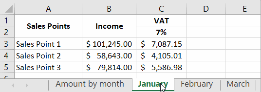
In the "Total per Month" sheet, construct a table to display the total income and tax for each month.
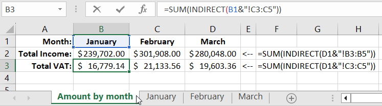
Attention! The column header names in cells B2:D2 should match the sheet names, which is essential for using the INDIRECT() function effectively, as it converts text into a cell reference.
=SUM(INDIRECT(B1&"!B3:B5"))
The ampersand symbol "&" concatenates two texts into one. Notice that the formula's parameters reference cell B2, which contains the month's name and the corresponding sheet name – "January." The text value of cell B2 is converted into a cell reference using the INDIRECT() function, resulting in the address of a three-dimensional reference: "January!B3:B5."
