How to use Absolute and Relative references in Excel

Microsoft Excel is a versatile analytical tool that allows you to perform calculations, find relationships between formulas, and carry out various mathematical operations efficiently.

The use of absolute and relative references in Excel simplifies a user's work. Relative references are notable for their address changing when copied, while absolute references maintain their addresses and values. We will also explore the benefits of mixed references and situations where they are indispensable.



How to Create an Absolute Reference in Excel

Often, you need to divide a total sum into parts. In such cases, the cell reference containing the total sum should not change in formulas when copied. This is where an absolute reference comes to your aid. How does an absolute reference look?

An absolute reference is represented with a dollar sign "$" preceding both the letter and the number.

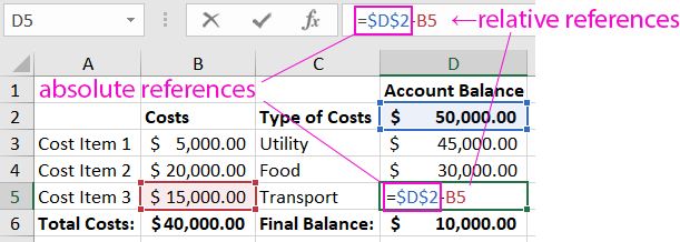
Regardless of copying to other cells, sheets, or workbooks, an absolute reference will always refer to the same column and row.

Handy tip! To add the "$" symbol automatically, use the F4 key when entering the reference.

If you need to change a relative reference to an absolute one:

1. Select the cell containing the formula you want to modify.
2. Go to the formula bar and place the cursor directly on the address.
3. Press "F4," and you'll see that Excel automatically offers different variations and adds the dollar sign.

4. Select the appropriate reference, occasionally pressing "F4," and then press "Enter."

This is a very convenient method that you should use frequently in your work.

Relative Cell Reference in Excel

By default, all references in Excel are relative. They look like this: =A2 or =B2 (only the number + letter):

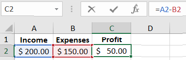
If we decide to copy this formula from row 2 to row 3, the addresses in the formula parameters will change automatically:

Relative references are convenient when you want to duplicate a similar calculation across multiple columns.

To use relative cells, follow these simple steps:

1. Select the cell you need.
2. Press Ctrl+C.
3. Select the cell where you want to insert the relative formula.
4. Press Ctrl+V.

Pro tip! If you have a similar calculation to perform, you can use a simple "life hack." Select the cell with the formula, then hover over the tiny square in the lower right corner to see a black cross. Drag the formula down, and Excel will automatically copy all values. This feature is called the AutoFill handle.

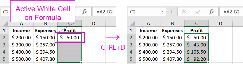
Even easier, select the range of cells where you need to apply formulas and ensure the active cell is on the formula, then press the Ctrl+D hotkey.

Download

Often, users need to change only the row or column reference while leaving the rest of the formula unchanged. To do this, Excel offers the concept of a "mixed reference."

How to Use a Mixed Reference in Excel

First, let's break it down. There are two types of mixed references:

Reference Type	Description
$A1	When you copy the formula vertically, the row number does not change.
A$1	When you copy the formula horizontally, the column letter does not change (e.g., A, B, C...).

To create a relative reference, you can use efficient methods. Of course, you can manually add the "$" symbol (switch to the English keyboard layout, then press SHIFT+4).

First, select the cell with the reference (or just the reference) and press "F4." The system will automatically suggest various options, and all that's left is to press "Enter."

Microsoft Excel offers a multitude of possibilities for its users. Therefore, it's essential to carefully study the examples and practice these techniques to streamline your work processes.