How to use VLOOKUP and MATCH to retrieve data in Excel

Not always are the tables created in Excel characterized by the fact that the category names of the data must be defined only in the column headers. Sometimes, when analyzing data tables, we have the option to use both column headers and row names located in the first column.



Example of a Formula with VLOOKUP and MATCH

An example of the original data table - a bonus table is shown below:

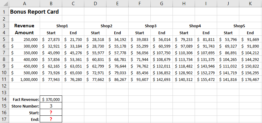
The purpose of this table is to search for corresponding bonus values in the range B5:K11 based on a specified revenue sum and store limits of minimum or maximum bonus payments. The complexity arises when automatically determining the bonus amount that an employee can expect when exceeding a certain revenue threshold. Since there is no clearly defined bonus payment amount for each possible revenue amount. There are only lower and upper limits of bonus amounts for each store.

For example, we need the program to automatically determine the possible minimum bonus for a seller from the 3rd store whose revenue has exceeded the level of 370,000.

For this:

1. Enter the revenue amount in cell B14: 370,000.
2. Specify the store number in cell B15: 3.
3. Enter the following formula in cell B16:

=VLOOKUP(B14,A5:K11,MATCH("Shop"&B15,A3:J3,0))

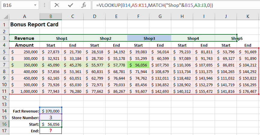
As a result, the lower threshold for the bonus is determined for store #3 when the revenue is greater than 370,000 but less than 400,000.

Searching for the Nearest Value Using Excel Formulas VLOOKUP and MATCH:

In the first argument of the VLOOKUP function, specify the reference to the cell with the search query (original revenue amount), which is in cell B14. The search area in the range A5:K11 is specified in the second argument of the VLOOKUP function. And the third argument must specify the column number, but it is currently unknown. From the second search query criterion, only the fact that the original column number relates to the 3rd store (cell B15) is known.

To determine the column number that contains the header "Shop 3", the MATCH function should be used. As the name of the function suggests, its task is to find the position where the value is located within a specified range of cells. In our case, we are looking for the value: "Shop 3", which should still be determined using the concatenation of the text string "Shop " and the criterion from cell B15. Therefore, in the first argument of the MATCH function, we specify "Shop"&B15. The second argument of the MATCH function specifies the reference to the viewed range A3:J3 where the original value (specified in the first argument) needs to be found. The third argument contains the value 0 - this means that the function will return the result as soon as it finds the first matching value. In our example, the value "Shop 3" is located at position number 6 in the range A3:J3, so the MATCH function returns the number 6, which will be used as the value for the third criterion of the VLOOKUP function. There is also a fourth argument in the VLOOKUP function that determines the accuracy of matching the found value to the query criterion (0 - exact match; 1 or empty - approximate match), but it is omitted in the formula for the following reason. After receiving all the arguments, the VLOOKUP function does not find the value 370,000, and since the last argument is not specified, it performs a search for the nearest value in Excel - 350,000.

Understanding the principle of the formula described above, based on it, you can easily compose a formula for automatically finding the maximum possible bonus for a seller from the 3rd store. The modified formula will be located in cell B17 and will have the following form:

=VLOOKUP(B14,A5:K11,MATCH("Shop"&B15,A3:J3,0)+1)

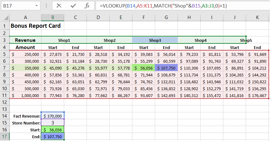
It is easy to notice that this formula differs from the previous one only in the column number specified in the third argument of the VLOOKUP function. Therefore, it is enough for us to add +1 to the value obtained through the MATCH function, as the maximum bonus amount is in the next column after the minimum amount corresponding to the search query criteria.

Download

Useful tips for formulas with VLOOKUP, INDEX, and MATCH functions:

To step-by-step analyze the formula of any complexity in Excel, it is rational to use the built-in tools in the section: "FORMULAS" - "Formula Auditing". For example, a particularly useful tool for step-by-step analysis of the computational cycle is "Evaluate Formula".

The VLOOKUP function searches for values from left to right in the specified range. That is, it analyzes cells only in columns located to the right relative to the first column of the original range specified in the first argument of the function. If the data arrangement structure in the table does not allow the VLOOKUP function to cover all columns for viewing for this reason, it is better to use a formula based on a combination of INDEX and MATCH functions.