Excel named ranges with absolute address tricks in Formulas
Most Excel users primarily employ one type of range name. When using a name in formulas, they refer to it as an absolute reference to a cell range. However, in the previous lesson, we assigned a name not to a range but to a value.
Advantages of Range Names Over Absolute References
Let's prepare a sheet where expenses are converted from one currency to another.
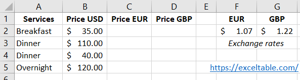
The conversion should be based on exchange rates that can change. Storing exchange rates directly in formulas is not ideal because changes would require edits in many cells.
For this task, we can use absolute references without range names, as shown below. However, names provide a more elegant solution. Let's compare both options.
Suppose we address the problem with an absolute reference to the cell containing the current exchange rate. We'd do the following:
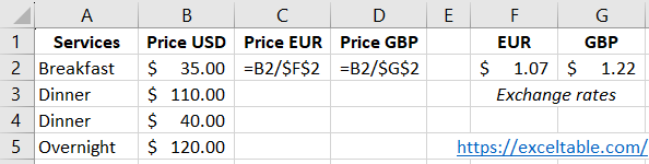
In cells C2 and D2, we enter formulas that refer to prices in rubles using relative references and to prices in other currencies using absolute references.
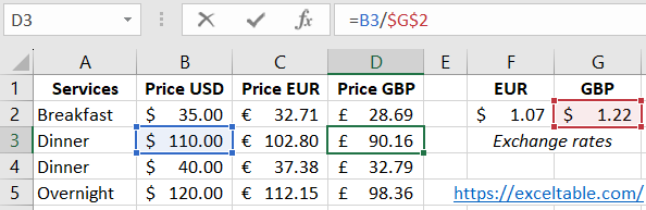
Such a solution works well for temporary calculations. The benefits of absolute references are clear; they recalculate a whole range of cells automatically when a single cell is updated.
The main disadvantage of absolute references is the reduced formula readability. In documents meant for long-term use, using names instead of absolute references improves readability. This greatly enhances a user's productivity when editing formulas to make adjustments or change the order of calculation arguments. It's especially important if the document is intended for a wide audience.
Automatic Creation and Addition of Excel Range Names in Formulas
Now, let's examine the advantages of using names for the task described above:
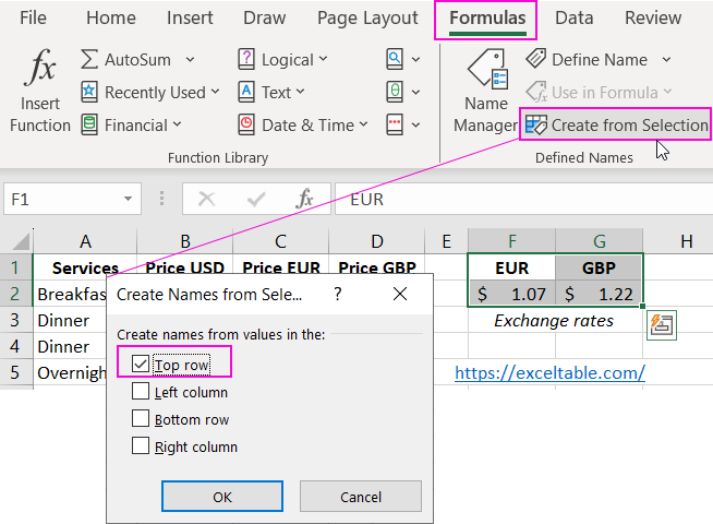
- Select the cell range F1:G2 and choose the "Formulas"-"Defined Names"-"Create from Selection" tool.
- In the "Create Names from Selection" dialog, choose the second option from the top, "Top row," as indicated in the image. This means that the values in the top rows will be used as the names for the cells in the bottom rows. Two names will be created simultaneously: cell F2 will be named "Euro," and cell G2 will be named "Dollar."
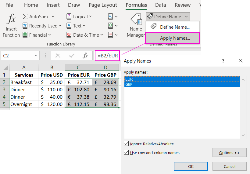
- Select the cell range C2:D5 and use the "Formulas"-"Defined Names"-"Assign Names"-"Apply Names" tool.
- In the dialog that appears, select the two names created earlier, and leave everything else as the default settings, then click "OK."
This is just a basic example of the benefits of using names instead of absolute references. With names, you can easily change exchange rates (by modifying the values in cells F2 and G2), and the prices will be updated automatically.
Note: Exchange rates can be stored not only in cell values but also directly in the names. Simply enter the current exchange rate in the "Refers to" field when creating the name.
Using Excel Names in Drop-Down Lists When Intersecting Sets
Now, let's provide a more illustrative example of the significant advantages of using names.
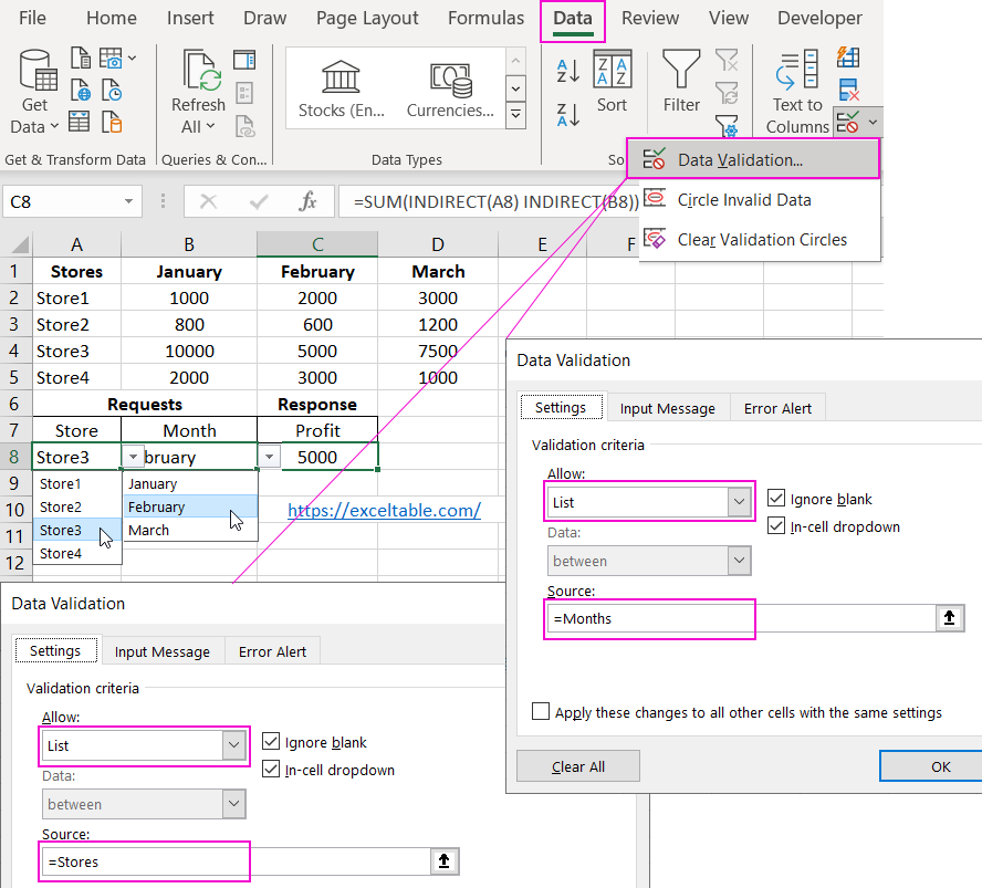
Create a sales report for the first quarter with data from four stores, as shown in the image:
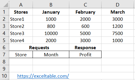
We will work with this report as if it were a database, using a formula and the intersection operator. In cells A8 and B8, we set up a query to the database, and in cell C8, we will receive the resulting answer. First, create all the necessary names:
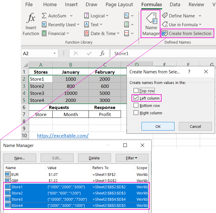
- Select the cell range A2:D5 and use the "Formulas"-"Create from Selection" tool. In the "Create Names from Selection" dialog, choose the second option from the top, "Left column."
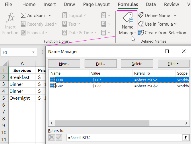
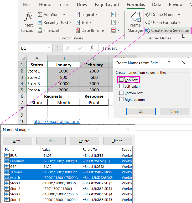
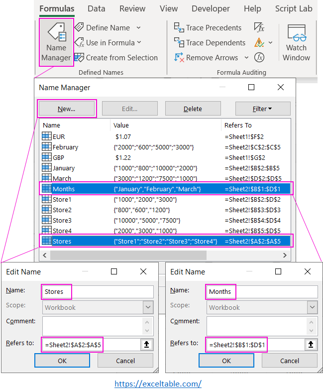
- Select the cell range B1:D1 and use the "Formulas"-"Create from Selection" tool. In the dialog, choose the second option from the top, "Top row." This way, we create all the names we need. To confirm, go to the "Name Manager" tool.
- Now, go to cell C8 and enter the SUM formula with the following arguments: =SUM(Store3 February) and press Enter.
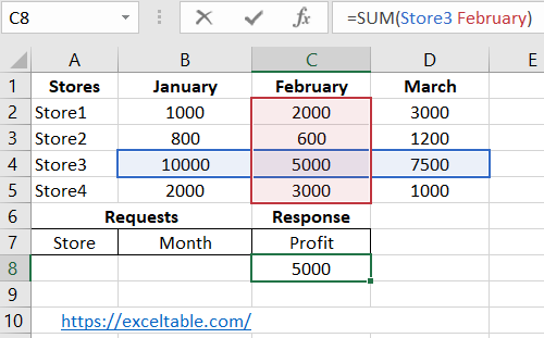
Great! The result is 500, which is the profit of Store 3 for February. Now, to create a query handler that also uses names in its algorithm:
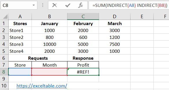
- Modify the formula in cell C8 as follows: =SUM(INDIRECT(A8) INDIRECT(B8)) and press Enter. The formula now returns an error: #REF!. Don't worry; we'll create the query handler next.
- Create two more names. Select the cell range A2:A5 and assign it the name "Stores." Select the cell range B1:D1 and assign it the name "Months."
- Create drop-down lists for error-free database queries. Go to cell A8 and use the "Data"-"Data Validation"-"Data Validation" tool. In the "Data Validation" dialog, adjust the settings as shown in the image, and click "OK."
- Create a second list with the months in cell B8 using the same approach.
 Download
Done! Now we can confidently work with our database. We specify the query parameters, and in cell C8, instead of the #REF! error, we see the correct result.
Note: Although lists are not necessary, as you can manually enter store and month names, using lists simplifies data entry and prevents potential errors when manually inputting values. The result will be the same.To some extent, this task could be solved without names using hard-to-read absolute cell reference addresses. However, implementing this query handler without using names would be much more challenging.
