VLOOKUP advanced formula with multiple conditions in Excel

Undoubtedly, it's easier to search through a single, albeit large, table or adjacent cell ranges than through multiple tables scattered across different non-adjacent ranges or even separate sheets. Even if you perform an automatic search simultaneously through multiple tables, significant obstacles can arise. Consolidating all data into one table is challenging and sometimes practically impossible. Let's demonstrate the correct solution for simultaneous search across multiple tables in Excel using a specific example.



Simultaneous Search Across Multiple Ranges

For a visual example, let's create three simple separate tables located in non-adjacent ranges on one sheet:

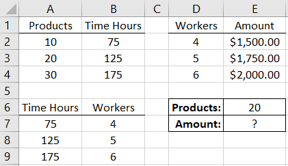
We need to search for the sum required to produce 20 units of a product. Unfortunately, this data is in different columns and rows. Therefore, we first need to check how much time is required for this production (first table).

Based on the obtained data, we need to proceed to the search in another table and find the number of workers needed for this production volume. The result obtained should be compared with the data in the third table. Thus, in one search operation across three tables, we will determine the required expenses (sum).

An average Excel user would seek a solution using formulas based on functions like VLOOKUP and would perform the search in three stages (separately for each table). However, it turns out you can get the ready-made result by performing the search in just 1 stage using a special formula. To do this:

1. In cell E6, enter the value 20, which is the condition for the search query.
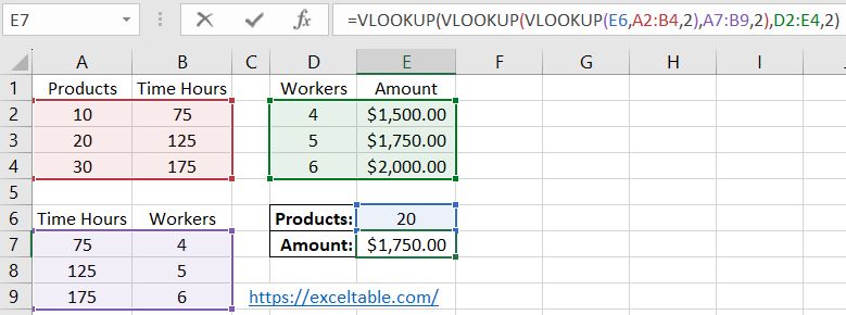
2. In cell E7, enter the following formula:

=VLOOKUP(VLOOKUP(VLOOKUP(E6,A2:B4,2),A7:B9,2),D2:E4,2)

Done!

Production cost for 20 units of a specific product.

How the Formula with VLOOKUP Works Across Multiple Tables

Download

The principle of this formula is based on the sequential search of all arguments for the main VLOOKUP function (the first one). First, the third VLOOKUP function searches for the amount of time required for production in the first table for the specified value in cell E6 (which can be changed as needed). Then, the second VLOOKUP function searches for the value for the first argument of the main function.

As a result of the third function's search, we get the value 125, which is the first argument for the second function. Having all parameters, the second function searches for the number of required workers in the second table for production. The result returned is 5, which will be further used by the main function. Based on all obtained data, the formula returns the final result of the calculation, namely, the sum of $1750 required for the production of 20 units of a specific product.

Following the same principle, you can use formulas for the VLOOKUP function from multiple sheets.